9 Formal Foundations: Trigonometric Derivatives and the Saddlepoint Test

Author

Gabriel J. Odom

Published

November 6, 2025

9.1 Overview

To prepare for the derivation of the Normal Distribution, we need a refresher on derivatives of trigonometric functions (and a few identities of trigonometric functions as well.) Also, for the maximum likelihood estimators that we’ve seen so far, the likelihood functions were either 1) univariate (having only one unknown parameter), like the Binomial or Exponential Distributions, or 2) bivariate (having two unknown parameters), but were so complicated that no closed form solution for the MLEs existed. However, for the Normal Distribution, we will have a bivariate likelihood (with both \(\mu\) and \(\sigma^2\) unknown), but we will be able get a closed-form system of two equations for these two unknowns which can be solved analytically. This means that we need a version of the Second Derivative Test that works for bivariate functions; this is called the Saddlepoint Test.

9.2 Trigonometric Functions and the Unit Circle

9.2.1 The Unit Circle

This is the Unit Circle, and it is crucial for our understanding of basic trigonometric functions.¹ The radius of the unit circle is 1, and we mostly use it to create right triangles² where the hypotenuse³ is the radius of the circle.

9.2.2 Sines and Cosines

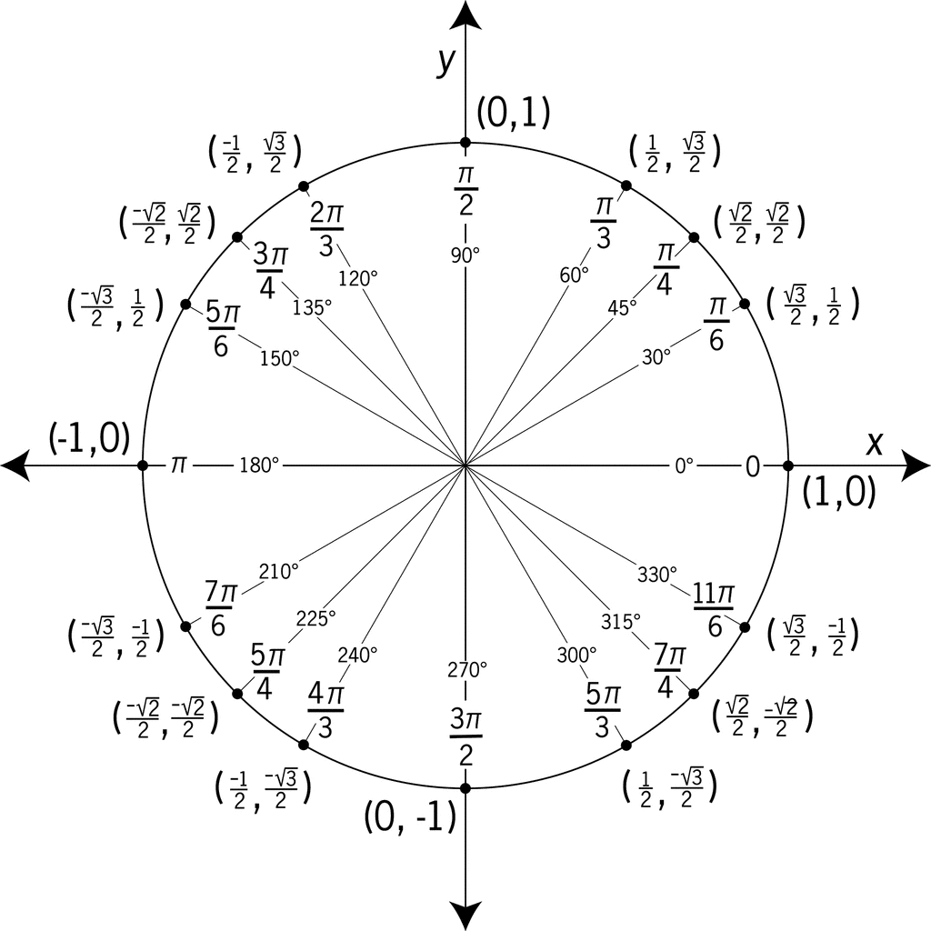
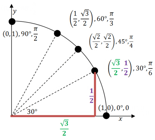
Let’s draw a triangle within this unit circle (image from this high school maths website).

We now have a right triangle from the origin to the edge of the unit circle. The sine function takes in the angle, often symbolized by \(\theta\), and returns the height of this triangle. Technically speaking, the sine function returns the ratio of the height of the triangle to its hypotenuse, but the hypotenuse of these triangles will be the radius of the unit circle, i.e. 1. The cosine function takes in this same angle and returns the width of this triangle. Because of this relationship, we often describe the unit circle relationship on the \(\langle x, y \rangle\) plane with \(x = \cos(\theta)\) and \(y = \sin(\theta)\). Also, applying the standard algebraic formula for a circle, we arrive at the most famous trigonometric identity⁴: \[ \begin{aligned} r^2 &= x^2 + y^2 \\ \Longrightarrow 1 &= x^2 + y^2 \\ \Longrightarrow 1 &= \cos^2(\theta) + \sin^2(\theta). \end{aligned} \]

The common mnemonic device to remember this is “SOH-CAH-TOA” (pronounced “sow kuh towuh” in American English):

Sine: Opposite side (height) divided by Hypotenuse

Cosine: Adjacent side (width) divided by Hypotenuse

Tangent: Opposite side (height) divided by Adjacent side (width)

Let’s calculate these values in R. Unfortunately, the trigonometric functions do not allow for input in degrees, so we must convert from degrees to radians.⁵ The formulae to convert between degrees and radians (and back) are \[ \text{Rad} = \text{Degrees}\times\frac{\pi}{180};\ \ \text{Degrees} = \text{Rad}\times\frac{180}{\pi}. \]

Let’s use the R sin() and cos() functions to confirm that a \(30^{\circ}\) triangle has a height of 0.5 and a width of \(\frac{1}{2}\sqrt{3}\):

Code

rads30_num <- 30 * pi / 180
sin(rads30_num)
[1] 0.5
cos(rads30_num)
[1] 0.866
sqrt(3)/2
[1] 0.866

One other important piece of information to know about these two functions is their graph over all \(360^{\circ}\) of a circle. Here is the sine:

Code

degrees_int <- 1:360
rads_num <- degrees_int * pi / 180
plot(
  x = degrees_int, y = sin(rads_num),
  main = "The Sine Function",
  xaxt = "n", xlab = "Degrees", ylab = "Sine"
)
axis(side = 1, at = seq(0, 360, by = 45))
abline(h = 0)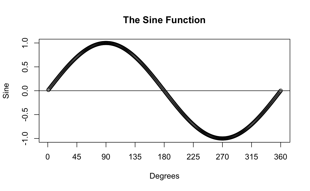

And here is the cosine:

Code

plot(
  x = degrees_int, y = cos(rads_num),
  main = "The Cosine Function",
  xaxt = "n", xlab = "Degrees", ylab = "Cosine"
)
axis(side = 1, at = seq(0, 360, by = 45))
abline(h = 0)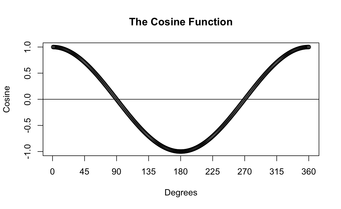

9.2.3 The Tangent Function

Now, there is one other main function in trigonometry that we mentioned but haven’t discussed: the tangent. From the calculus perspective, the term “tangent” refers to a straight line with the slope that’s equal to a curve at a particular point. For a refresher, go back to the Formal Foundations section on the Limit Definition of the Derivative in the Poisson Distribution lesson. For trigonometry, the term “tangent” refers to a function relating the angle of a triangle to the ratio of its height and width. Using R, let’s confirm that this ratio for this triangle above is \((1/2) \div (\frac{1}{2}\sqrt{3})\):

Code

tan(rads30_num)
[1] 0.577
(1/2) / (sqrt(3)/2)
[1] 0.577

Recall that the width of these triangles will oscillate from a maximum of 1 (when the angle is a multiple of \(180^{\circ}\)) to a width of 0 (when the angle is half of a multiple of \(180^{\circ}\)). Therefore, because the tangent is defined by the ratio of height to width, the tangent will be undefined (due to division by 0) when when the angle is half of a multiple of \(180^{\circ}\). Let’s plot the tangent as well:

Code

plot(
  x = degrees_int, y = tan(rads_num), ylim = c(-5, 5),
  main = "The Tangent Function",
  xaxt = "n", xlab = "Degrees", ylab = "Tangent"
)
axis(side = 1, at = seq(0, 360, by = 45))
abline(v = c(90, 270))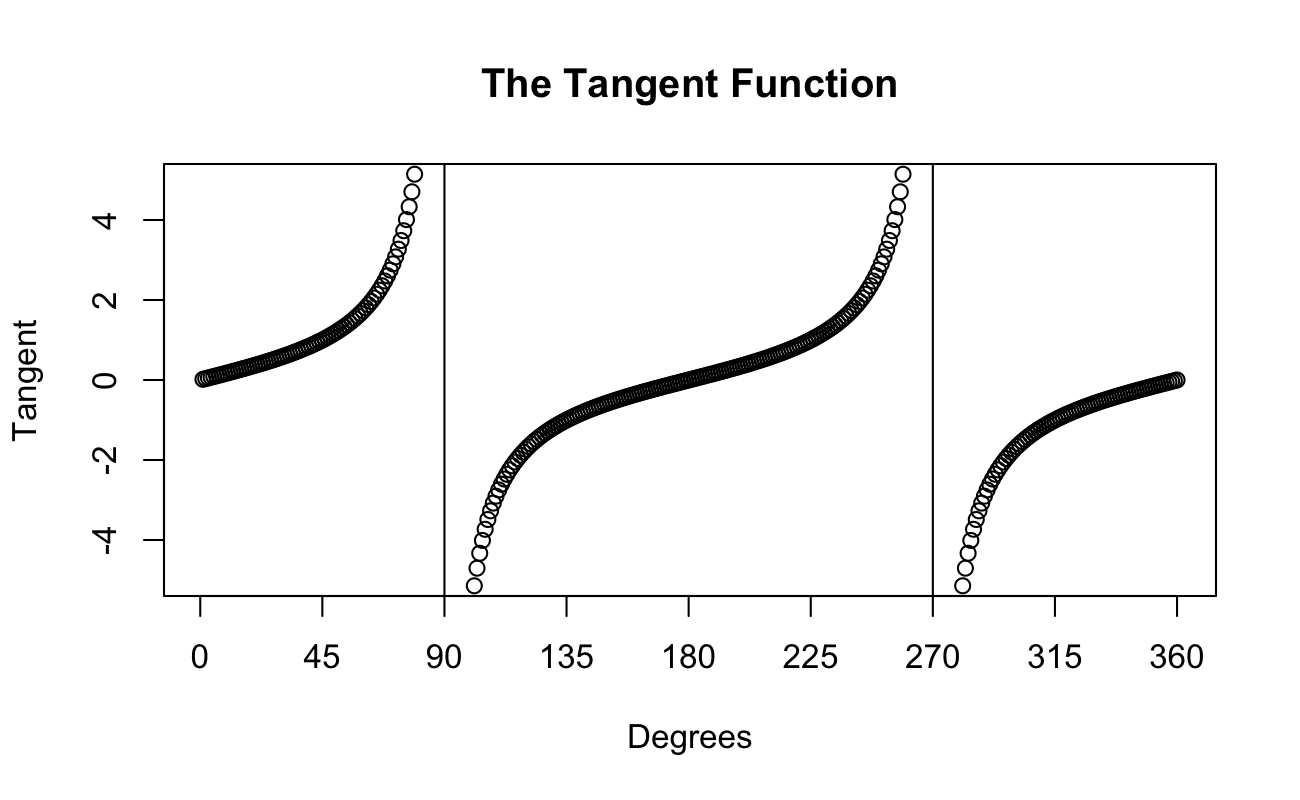

9.2.4 Inverse Trigonometric Functions

As with almost all mathematical operators, the trigonometric functions have inverse functions.⁶ These are functions that “undo” the effects of the original function. For example, if \(f(x) = \sqrt{x}\), then \(g(x) = x^2\) “undoes” the effects of \(f\). For the trigonometric functions, these inverse functions are called the “arc” functions and defined as follows: \[ \begin{aligned} \arcsin(\sin(\theta)) &= \theta, \\ \arccos(\cos(\theta)) &= \theta, \\ \arctan(\tan(\theta)) &= \theta. \end{aligned} \] So, these “arc” functions “undo” their corresponding trigonometric functions. These often come up when solving equations for an angle \(\theta\). For example: \[ \begin{aligned} \sin(\theta) &= \frac{\text{height}}{\text{radius}} \\ \Longrightarrow \arcsin(\sin(\theta)) &= \arcsin\left( \frac{\text{height}}{\text{radius}} \right) \\ \Longrightarrow \theta &= \arcsin\left( \frac{\text{height}}{\text{radius}} \right). \end{aligned} \]

We will also graph these three functions, but we remark that their domains will be different. For sine and cosine, the domain was \([0^{\circ}, 360^{\circ}]\); the range was \([-1,1]\). For tangent, the domain was \([0^{\circ}, 360^{\circ}]\) except for the vertical asymptotes at \(\{90^{\circ}, 270^{\circ}\}\); the range was \((-\infty, \infty)\). Also, as before, R uses radians instead of degrees, so we will also have to transform back the results to degrees.

Let’s plot these inverse trigonometric functions, but pay special attention to their domains and ranges. Let’s start with the arcsine (using the asin() function):

Code

triangleHeights_num <- seq(-1, 1, length.out = 101)
thetaRads_num <- asin(triangleHeights_num)
plot(
  x = triangleHeights_num, y = 180 * thetaRads_num / pi, ylim = c(-90, 90),
  main = "The Arcsine Function",
  xaxt = "n", xlab = "Triangle Heights",
  yaxt = "n", ylab = "Generating Angle"
)
axis(side = 1, at = seq(-1, 1, length.out = 9))
axis(side = 2, at = seq(-90, 90, by = 30))
abline(h = 0)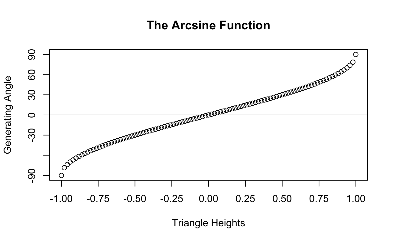

Similarly, we can plot the arccosine (using the acos() function):

Code

triangleWidths_num <- seq(-1, 1, length.out = 101)
thetaRads_num <- acos(triangleWidths_num)
plot(
  x = triangleWidths_num, y = 180 * thetaRads_num / pi, ylim = c(0, 180),
  main = "The Arccosine Function",
  xaxt = "n", xlab = "Triangle Widths",
  yaxt = "n", ylab = "Generating Angle"
)
axis(side = 1, at = seq(-1, 1, length.out = 9))
axis(side = 2, at = seq(0, 180, by = 30))
abline(h = 0)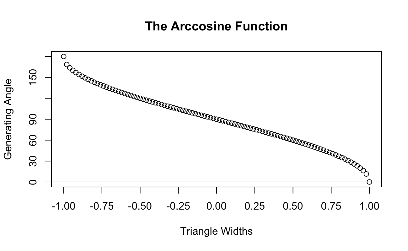

Finally, for the arctangent, because this function takes the ratio of triangle heights and widths as its input, the domain of possible values includes the entire Real line. However, the range of the function is only from \((-90^{\circ}, 90^{\circ})\) (or \(-\frac{\pi}{2}\) to \(\frac{\pi}{2}\) in radians). We now plot the this function (using the atan() function):

Code

triangleTan_num <- seq(-4, 4, length.out = 81)
thetaRads_num <- atan(triangleTan_num)
plot(
  x = triangleTan_num, y = 180 * thetaRads_num / pi, ylim = c(-90, 90),
  main = "The Arctangent Function",
  xaxt = "n", xlab = "Triangle (Height / Width)",
  yaxt = "n", ylab = "Generating Angle"
)
axis(side = 1, at = seq(-4, 4, length.out = 9))
axis(side = 2, at = seq(-180, 180, by = 45))
abline(h = 0)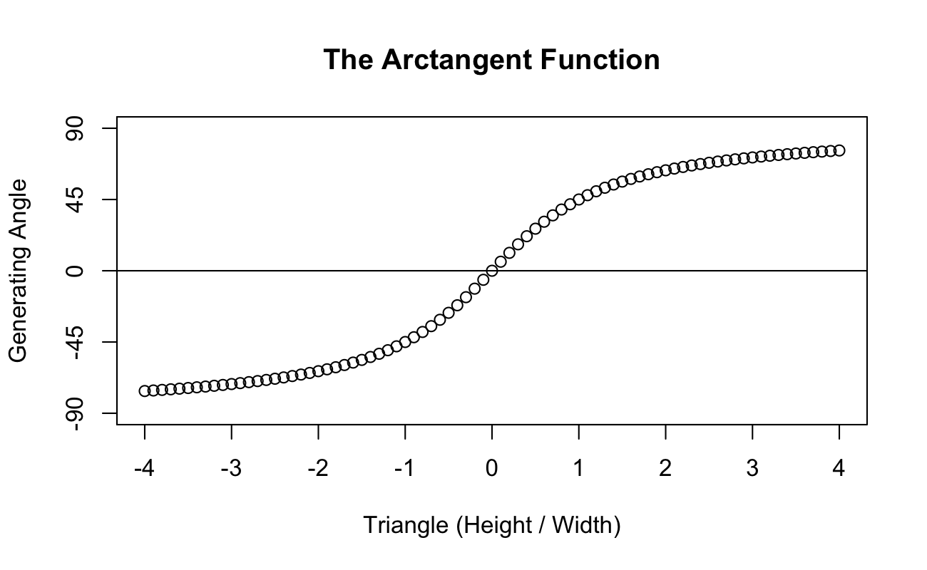

9.3 Trigonometric Derivatives

Now that we’ve had a basic refresher on the trigonometric functions, we want to get some intuition for the well-known trigonometric derivatives. These derivatives are \[ \begin{aligned} \frac{d}{d\theta} \sin(\theta) &= \cos(\theta), \\ \frac{d}{d\theta} \cos(\theta) &= -\sin(\theta), \\ \frac{d}{d\theta} \tan(\theta) &= 1 + \tan^2(\theta). \end{aligned} \]

9.3.1 Derivatives of Sine and Cosine

Rather than going through the deep dive⁷ needed to prove these derivatives, we will simply plot the slope of the sine function at many very small intervals. First, recall the graph of the sine (this time in radians):

Code

plot(
  x = rads_num, y = sin(rads_num),
  main = "The Sine Function",
  xaxt = "n", xlab = "Radians", ylab = "Sine"
)
axis(side = 1, at = seq(0, 2*pi, by = pi/4))
abline(h = 0)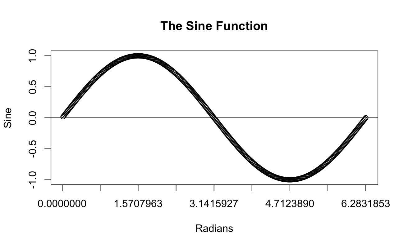

We already see that the slope at 0 is 1, the slope at \(\pi/2\) is 0, the slope at \(\pi\) is negative 1, the slope at \(3\pi/2\) is 0 again, and the slope at \(2\pi\) is 1 again. (Also, since we don’t care about the angles themselves, I’m going to leave the computing in radians. It won’t matter to the shape of the curve.) Here are those points plotted (with the cosine curve in green):

Code

plot(
  x = seq(0, 2 * pi, length.out = 5), y = c(1, 0, -1, 0, 1),
  xaxt = "n", xlab = "Radians", xlim = c(0, 2*pi),
  yaxt = "n", ylab = "Slopes", ylim = c(-1, 1),
  main = "Slopes of the Sine Function"
)
axis(side = 1, at = seq(0, 2*pi, by = pi/4))
axis(side = 2, at = seq(-1, 1, by = 0.5))
curve(cos(x), add = TRUE, col = "darkgreen", lwd = 2)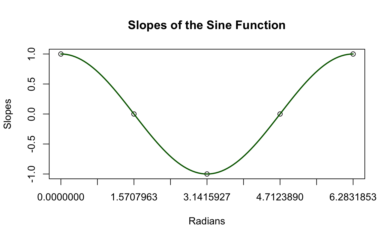

Let’s write a function to calculate these slopes at more than these five simple points. (And we want the computer to calculate slopes for us.) I’m going to start very “rough”, and evaluate the slope at only 9 points:

Code

nPoints_int <- 9
radsSparse_num <- seq(0, 2 * pi, length.out = nPoints_int + 1)
sineSlopes_num <- vector(mode = "numeric", length = nPoints_int)
midpoints_num <- vector(mode = "numeric", length = nPoints_int)

for (x in seq_len(nPoints_int)) {
  
  deltaY <- sin(radsSparse_num[x + 1]) - sin(radsSparse_num[x])
  deltaTheta <- radsSparse_num[x + 1] - radsSparse_num[x]
  
  sineSlopes_num[x] <- deltaY / deltaTheta
  midpoints_num[x]  <- (radsSparse_num[x + 1] + radsSparse_num[x]) / 2
  
}

plot(
  x = midpoints_num, y = sineSlopes_num,
  xaxt = "n", xlab = "Radians", xlim = c(0, 2*pi),
  yaxt = "n", ylab = "Slopes", ylim = c(-1, 1),
  main = "Slopes of the Sine Function"
)
axis(side = 1, at = seq(0, 2*pi, by = pi/4))
axis(side = 2, at = seq(-1, 1, by = 0.5))
curve(cos(x), add = TRUE, col = "darkgreen", lwd = 2)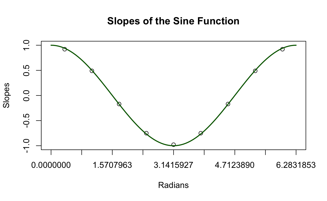

Because the computer is doing all the work, let’s increase to 99 points:

Code

nPoints_int <- 99
radsSparse_num <- seq(0, 2 * pi, length.out = nPoints_int + 1)
sineSlopes_num <- vector(mode = "numeric", length = nPoints_int)
midpoints_num <- vector(mode = "numeric", length = nPoints_int)

for (x in seq_len(nPoints_int)) {
  
  deltaY <- sin(radsSparse_num[x + 1]) - sin(radsSparse_num[x])
  deltaTheta <- radsSparse_num[x + 1] - radsSparse_num[x]
  
  sineSlopes_num[x] <- deltaY / deltaTheta
  midpoints_num[x]  <- (radsSparse_num[x + 1] + radsSparse_num[x]) / 2
  
}

plot(
  x = midpoints_num, y = sineSlopes_num,
  xaxt = "n", xlab = "Radians", xlim = c(0, 2*pi),
  yaxt = "n", ylab = "Slopes", ylim = c(-1, 1),
  main = "Slopes of the Sine Function"
)
axis(side = 1, at = seq(0, 2*pi, by = pi/4))
axis(side = 2, at = seq(-1, 1, by = 0.5))
curve(cos(x), add = TRUE, col = "darkgreen", lwd = 2)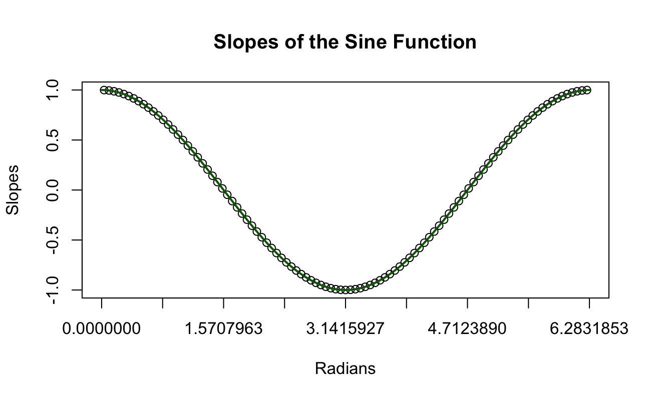

As we can see, as the difference between each angle shrinks (i.e. as \(\Delta\theta \to 0\)), the slopes of the lines tangent to the sine function approach the values given by the cosine function. Not to belabour the point, but we can apply the exact same effort to show that the derivative of the cosine function is \(-1\) times the sine function. This line of reasoning is not a proof (for a formal proof, see the link to Prof. Brown’s notes that I also included in the footnote above), but it does help us understand what is going on a bit better.

9.3.2 Derivative of Tangent

Now that we have the derivative of \(\sin(\theta)\) and \(\cos(\theta)\), the derivative of \(\tan(\theta)\) is far more straightforward, using the Quotient Rule and the two derivatives we just reviewed: \[ \begin{aligned} \frac{d}{d\theta} \tan(\theta) &= \frac{d}{d\theta} \frac{\sin(\theta)}{\cos(\theta)} \\ &= \frac{\cos(\theta) \frac{d}{d\theta} \sin(\theta) - \sin(\theta) \frac{d}{d\theta} \cos(\theta)}{[\cos(\theta)]^2} \\ &= \frac{\cos(\theta) \times [\cos(\theta)] - \sin(\theta) \times [-\sin(\theta)]}{\cos^2(\theta)} \\ &= \frac{\cos^2(\theta) + \sin^2(\theta)}{\cos^2(\theta)} \\ &= \frac{\cos^2(\theta)}{\cos^2(\theta)} + \frac{\sin^2(\theta)}{\cos^2(\theta)} \\ &= 1 + \tan^2(\theta). \end{aligned} \]

9.3.3 Derivative of the Arctangent

This derivative is more non-traditional (that is, creative). Let’s begin by letting \(\arctan(x) = \theta\), which implies that \(\tan(\theta) = x\). Then,⁸ \[ \begin{aligned} \frac{d}{dx} \tan(\theta) &= \frac{d}{dx}x \\ \qquad\text{\emph{Chain rule...}}& \\ \Longrightarrow \left( 1 + \tan^2(\theta) \right) \frac{d\theta}{dx} &= 1 \\ \left( 1 + [\tan(\theta)]^2 \right) \frac{d[\theta]}{dx} &= 1 \\ \qquad\text{\emph{Substitute back in...}}& \\ \left( 1 + [x]^2 \right) \frac{d[\arctan(x)]}{dx} &= 1 \\ \Longrightarrow \frac{\left( 1 + x^2 \right)}{\left( 1 + x^2 \right)} \frac{d}{dx}\arctan(x) &= \frac{1}{1 + x^2} \\ \Longrightarrow \frac{d}{dx}\arctan(x) &= \frac{1}{1 + x^2}. \end{aligned} \]

9.4 The Saddlepoint Test

As a comment, parts of this “Formal Foundations” section requires a foundational understanding of vectors and linear algebra, which is well beyond the scope of this text. For a primer on linear algebra, I recommend Prof. Gilbert Strang’s MIT Linear Algebra course here: https://ocw.mit.edu/courses/18-06-linear-algebra-spring-2010/. It’s completely free, but it will take you a few weeks to get through it all.

9.4.1 Introduction

When we find the maximum likelohood estimators, we were careful to also check the second derivatives to ensure that those derivatives were negative at our candidate points for the MLEs (these candidate values are the solution points to the systems of first order partial derivatives, also known as critical points⁹). In the simple \(x,y\) (2-dimensional) plane for introductory calculus, for some critical point \(x_0\), checking if \(x_0 \ni f^{\prime}(x_0) = 0\) was a minimum or maximum was often quite simple (and we will go over a refresher example below). This is because changes could only ever be in one dimension: along \(x\).

However, for a function in higher dimensions, such as \(z = f(x,y)\), changes can happen in infinitely many directions, as long as they are some combination of changes in \(x\) and \(y\). We can’t simply check the derivatives along the \(x\) axis or the \(y\) axis only; we also have to check the infinitely many derivatives across every direction between \(x\) and \(y\). This already sounds like a problem, and we’ve only described a simple surface in 3 dimensions!

Instead of trying to walk through uncountably infinitely many partial derivatives in every direction around a critical point, we will use the geometric properties of the likelihood function instead. If we have found a point where the gradient¹⁰ of \(f\) equals 0, then there are a few options:

\(f\) is concave up, and the point is a local minimum,
\(f\) is concave down, and the point is a local maximum,
around the point, \(f\) is increasing in some directions and decreasing in others, so the point is a saddlepoint¹¹, or
\(f\) is not second-order differentiable at the point (which means you’re in trouble). We won’t really cover this last option for our work in optimizing likelihood functions, but it is theoretically possible.

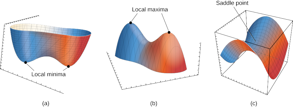
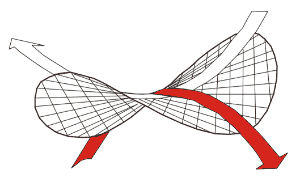
One beneficial heuristic to understanding these shapes is to check for their ability to “hold water”. In the figure above, the shapes in (a) and (b) could be rotated around to eventually serve as a bowl of some kind. For part (a), the figure stays the same; for part (b), we would have to flip it over. However, in part (c), we notice that no possible rotation exists for the shape to hold water. Therefore, the figures in parts (a) and (b) have local extrema at their critical points, but the figure in part (c) has a saddlepoint.

9.4.2 Two-Dimensional Use Case

Let’s take a step back and look at an example on the \(x,y\) plane. We have a function \(f\), and we will take its first two derivatives: \[ \begin{aligned} f(x) &= x^3 - 3x + 2 \\ f^{\prime}(x) &= 3x^2 - 3 \\ f^{\prime\prime}(x) &= 6x. \end{aligned} \] We set our first derivative equal to 0 to find the critical points: \[ \begin{aligned} 0 &\overset{\text{set}}{=} 3x^2 - 3 \\ \Longrightarrow 0 &= x^2 - 1 \\ &= (x - 1)(x + 1) \\ \Longrightarrow x &= \{-1, 1\}. \end{aligned} \] If we were doing statistics or biostatistics, many students at this point would shout and say “I’ve found the maximum!” or “I’ve found the minimum!”—which ever one they were looking for in the first place. Well, let’s graph this function to find out:

Code

domain_num <- seq(-3, 3, length.out = 101)
f_num <- (domain_num)^3 - 3*(domain_num) + 2

plot(
  x = domain_num, y = f_num,
  main = "", xlab = "x", ylab = "y"
)

It appears that we have a local maxima at \(x = -1\) and a local minima at \(x = 1\). However, many real problems are not so easy, as we’ve seen in this class. For example, in our statistical distributions, the parameters were arbitrary, not fixed numbers, so there would be no way to graph the likelihood anyway. We need analytical solutions.

9.4.3 The First Derivative Test

How do we know that what the critical point we’ve found is a maximum? (Or minimum?) We need to know what’s happening to \(f\) near these two points. Let \(x^*\) denote the \(x\) values of our critical points. Here are our two decision schemes:

The First Derivative Test

If where \(x < x^*\), the derivative is negative, AND, where \(x > x^*\), the derivative is positive, then \(x^*\) is a minima of \(f\).

If where \(x < x^*\), the derivative is positive, AND, where \(x > x^*\), the derivative is negative, then \(x^*\) is a maxima of \(f\).

If the derivative has the same sign on both sides of \(x^*\), then the critical value is neither a minima nor a maxima.

Here’s an example from some undergrad worksheet (this text uses critical number instead of critical value, but they mean the same thing; also I have no idea what textbook this is from to be honest).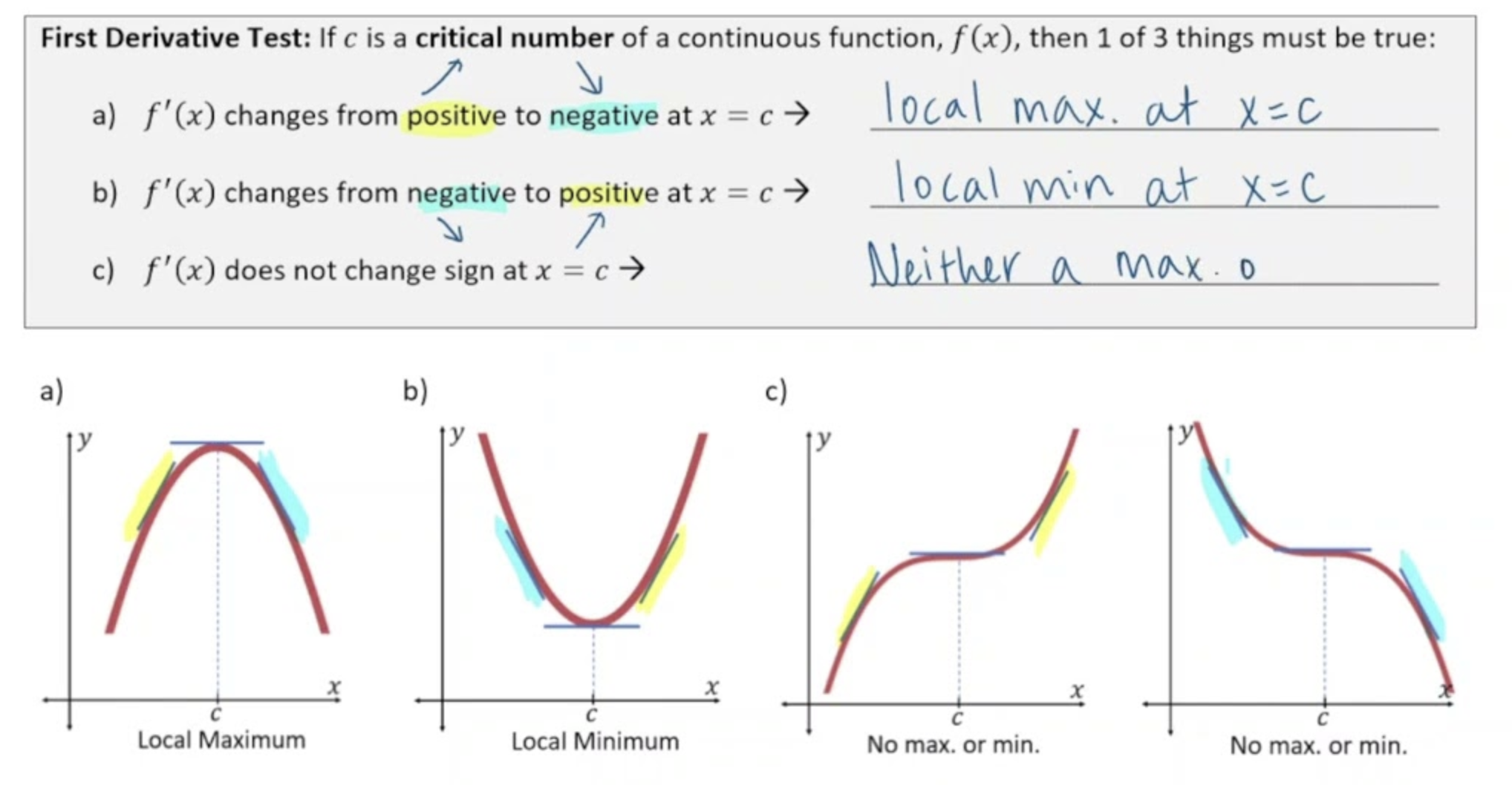

For our function \(f\) above:

\(f^{\prime}(-2) = 3(-2)^2 - 3 = 3(4) - 3 = 9 > 0\), so \(f\) is increasing for \(x < -1\),
\(f^{\prime}(0) = -3\), so \(f\) is decreasing for \(-1 < x < 1\), and
\(f^{\prime}(2) = 3(2)^2 - 3 = 3(4) - 3 = 9 > 0\), so \(f\) is increasing for \(x > 1\).

Therefore, \(f\) is increasing on the left side and decreasing on the right side of \(x^* = -1\), so this critical point is a local maximum. Additionally, \(f\) is decreasing on the left side and increasing on the right side of \(x^* = 1\), so this critical point is a local minimum.

9.4.4 The Second Derivative Test

There is another option to find if a critical point is a minimum/maximum/neither (in case you think that plugging in values all around the critical points is tedious). The second derivative test checks the concavity¹² of \(f\) around critical values. Imaging rain falling on our function \(f\); think about concavity as the ability to “hold” the rainwater (concave up, like a bucket) or “shelter” from the rainwater (concave down, like an umbrella).¹³

The Second Derivative Test

If \(f^{\prime\prime}(x^*) > 0\), then \(f\) is concave up at \(x^*\), and this point is a minima of \(f\).

If \(f^{\prime\prime}(x^*) < 0\), then \(f\) is concave down at \(x^*\), and this point is a maxima of \(f\).

If \(f^{\prime\prime}(x^*) = 0\), then the critical value is neither a minima nor a maxima.

Here is another visual aide (from some other unknown calculus textbook):

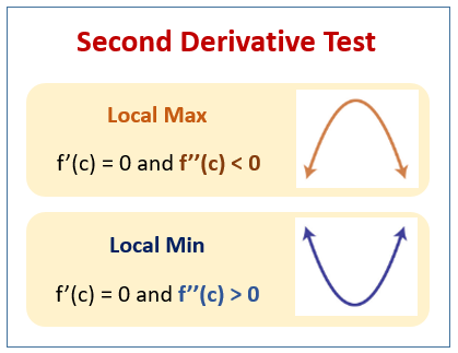
For our function \(f\) above:

\(f^{\prime\prime}(-1) = 6(-1) = -6 < 0\), so \(f\) is concave down at \(x = -1\), so this critical point is a local maximum.
\(f^{\prime\prime}(1) = 6(1) = 6 > 0\), so \(f\) is concave up at \(x = 1\), so this critical point is a local minimum.

9.4.5 Extending to Higher Dimensions

The work that we’ve done so far is great if we have our response as a function of a single predictor (like \(y = f(x)\)). But many of the likelihoods we’ve encountered so far have two or more unknown parameters. What happens then?

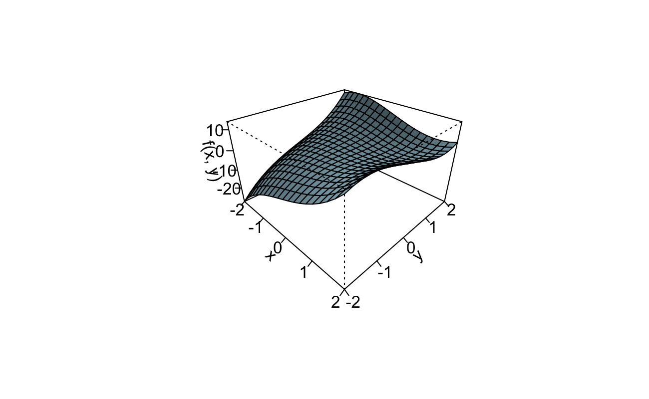
Let’s start with a simple function in 3 dimensions (ChatGPT helped me come up with this): \[ f(x,y) = x^3 + y^3 - 3xy. \]

What does it look like? Can we clearly tell where any minima/maxima are?

Code

# Define the function
f <- function(x, y) {
  x^3 + y^3 - 3*x*y
}

# Create a grid of x and y values
x <- seq(-2, 2, length.out = 20)
y <- seq(-2, 2, length.out = 20)
z <- outer(x, y, f)

# Create the perspective plot
persp(
  x, y, z,
  theta = 45, phi = 30,    # Viewing angles
  expand = 0.6,            # Zoom
  col = "lightblue",       # Surface color
  xlab = "x", ylab = "y", zlab = "f(x, y)",
  ticktype = "detailed",   # Detailed axis ticks
  shade = 0.5              # Shading for depth
)

We should start by taking some derivatives. \[ \begin{aligned} \frac{\partial}{\partial x} f(x,y) &= 3x^2 - 3y \\ \frac{\partial}{\partial y} f(x,y) &= 3y^2 - 3x. \end{aligned} \] Setting these equations to 0 yields the following system (I also divide out the 3): \[ \begin{aligned} 0 &= x^2 - y \Rightarrow y = x^2 \\ 0 &= y^2 - x \Rightarrow y = \pm\sqrt{x}. \end{aligned} \] Let’s equate these.

First take the option for \(y = -\sqrt{x}\). Where is \(x^2 = -\sqrt{x}\)? Only at \(x = 0\). Therefore \(\{x = 0, y = 0\}\) are the \(x,y\) coordinates of a critical point of \(f(x,y)\). At this point, \(f(0,0) = 0\), so the candidate critical 3-tuple¹⁴ is \(\langle 0, 0, 0 \rangle\).
Now take the option for \(y = \sqrt{x}\). Where is \(x^2 = \sqrt{x}\)? We should quickly see by substitution that this is only true when \(x \in \{0,1\}\). However, we will also show it analytically: \[ \begin{aligned} x^2 &= \sqrt{x} \\ \Rightarrow x^4 &= x \\ \Rightarrow x^4 - x &= 0 \\ \Rightarrow x(x^3 - 1) &= 0. \end{aligned} \] Thus, \(x = 0\) and \(x^3 = 1 \Rightarrow x = 1\). Subsequently, \(y = 0\) and \(y = 1\). Therefore, at these points, the \(f\) values are: \[ f(0,0) = 0;\ \ f(1,1) = 1 + 1 - 3(1)(1) = -1. \] Hence, the critical 3-tuples are \(\langle 0, 0, 0 \rangle\) (which we saw above), and \(\langle 1, 1, -1 \rangle\).

9.4.6 “Holding Water”

One of the best ways I’ve found to understand the shape of surfaces in higher dimensions is to think about a rain shower falling from above onto the surface. If there is a region that water can “pool” (collect) in, then there will be at least one local minimum in that region. Similarly, if I flip the surface upside down, and I then get a region for water to pool in, then the original surface has at least one local maximum in that region. Finally, if the water never collects in a region, even if I flip the surface upside down, then that region does not have any local extrema.

Let’s go back to our graph of \(f(x) = x^3 - 3x + 2\):

Code

domain_num <- seq(-3, 3, length.out = 101)
f_num <- (domain_num)^3 - 3*(domain_num) + 2

plot(
  x = domain_num, y = f_num,
  main = "", xlab = "x", ylab = "y"
)

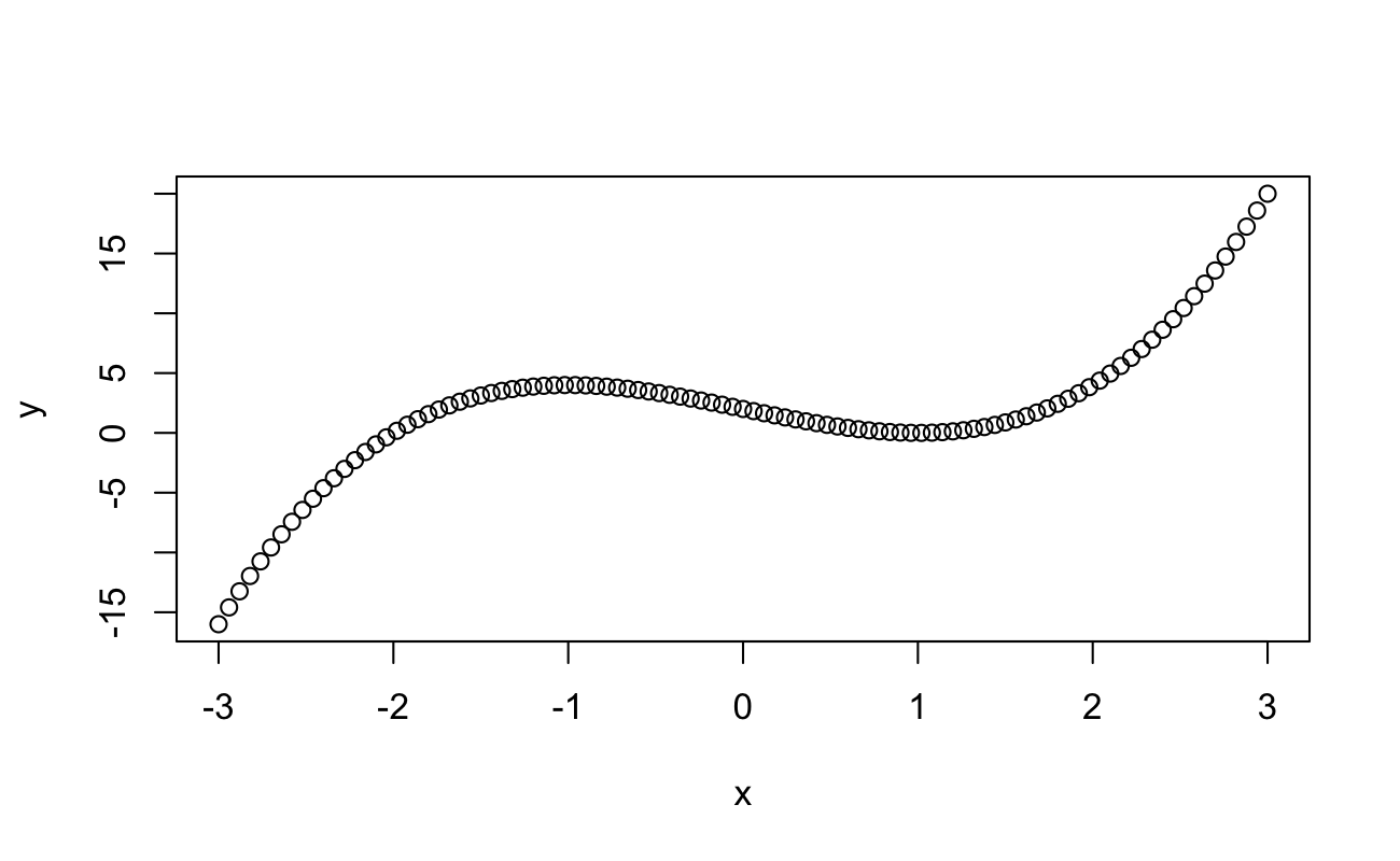
If I allow rain to fall on \(f\) from “above”, then water will collect in a pool around the point \(x = 1\); this point is a local minimum of \(f\). If allow rain to fall on \(-f\) from above (where I’ve flipped \(f\) over vertically), then water will collect in a pool around the point \(x = -1\); this point is a local maximum of \(f\).

This example of “holding water” extends easily to higher dimensions. If, around a point in \(\mathbb{R}_p\), the surface forms a “bowl” shape, then there will be a local minimum. If, around a point in \(\mathbb{R}_p\), the surface forms an “umbrella” shape, then there will be a local maximum. The way that we measure if a higher dimensional shape has “volume” is with the determinant¹⁵ For clarity, both bowl and umbrella shapes can hold some water in them, but we make a fancy abstraction and say that the umbrella holds “negative” water—that is, that it would hold water if you flipped it upside down.

9.4.7 The Hessian Matrix

The Hessian Matrix¹⁶ is a matrix of all the second-order partial derivatives of a function. The “volume” of this matrix at a point in \(\mathbb{R}_p\) will tell us if \(f\) has a bowl shape, an umbrella shape, or no water-holding shape at all at that point. Again, we measure the volume of a matrix by calculating the determinant.

The Hessian Determinant and Saddlepoint Test

Let \(\textbf{H}\) be the Hessian Matrix of all second-order partial derivatives of \(f:\mathbb{R}_p \to \mathbb{R}\). As long as \(\det\{\textbf{H}[f(\textbf{x})]\} > 0\), then \(f\) has volume at this point (but we won’t know if it’s positive or negative volume). To check if the volume is positive or negative, we look at the second derivative in any direction. Why? Because a bowl is increasing every direction and an umbrella is decreasing in every direction, so once we know \(f\) has a bowl/umbrella shape, it doesn’t matter which second derivative we look at. Here are the decision rules:

If \(\det\{\textbf{H}[f(\textbf{x})]\} > 0\) at the point \(\textbf{x}\), then we check if the diagonals are positive:

If so, then \(f\) is concave up (\(f\) would collect water around this point) and \(\textbf{x}\) is a local minimum.

If not, then \(f\) is concave down (-\(f\) would collect water around this point, but \(f\) would act like an umbrella there) and \(\textbf{x}\) is a local maximum.

If \(\det\{\textbf{H}[f(\textbf{x})]\} < 0\) at the point \(\textbf{x}\), then \(\textbf{x}\) is called a saddlepoint of \(f\). The point \(\textbf{x}\) is neither a minimum nor a maximum.

If \(\det\{\textbf{H}[f(\textbf{x})]\} = 0\) at the point \(\textbf{x}\), then the saddlepoint test is inconclusive (and you’re in trouble).

Let’s go back to our 3-D function, \(f(x,y) = x^3 + y^3 - 3xy\). Using the first derivatives, we found that \(\langle 0, 0, 0 \rangle\) and \(\langle 1, 1, -1 \rangle\) are critical points of the function \(f\). Now let’s calculate the Hessian. Recall that: \[ \begin{aligned} \frac{\partial}{\partial x} f(x,y) &= 3x^2 - 3y \\ \frac{\partial}{\partial y} f(x,y) &= 3y^2 - 3x. \end{aligned} \] Therefore, \[ \begin{aligned} \textbf{H}[f(x,y)] &= \begin{bmatrix} \frac{\partial}{\partial x} \frac{\partial f}{\partial x} & \frac{\partial}{\partial x} \frac{\partial f}{\partial y} \\ \frac{\partial}{\partial y} \frac{\partial f}{\partial x} & \frac{\partial}{\partial y} \frac{\partial f}{\partial y} \end{bmatrix} \\ &= \begin{bmatrix} \frac{\partial}{\partial x} 3x^2 - 3y & \frac{\partial}{\partial x} 3y^2 - 3x \\ \frac{\partial}{\partial y} 3x^2 - 3y & \frac{\partial}{\partial y} 3y^2 - 3x \end{bmatrix} \\ &= \begin{bmatrix} 6x & -3 \\ -3 & 6y \end{bmatrix}. \end{aligned} \]

The first critical point was \(\{x = 0, y = 0\}\). Let’s check the determinant¹⁷ at this point: \[ \begin{aligned} \textbf{H}[f(0,0)] &= \begin{bmatrix} 6[0] & -3 \\ -3 & 6[0] \end{bmatrix} \\ &= \begin{bmatrix} 0 & -3 \\ -3 & 0 \end{bmatrix} \\ \Longrightarrow \det\{\textbf{H}[f(0,0)]\} &= [0][0] - [-3][-3] \\ &= -9. \end{aligned} \] Therefore, the surface given by \(f(x,y)\) is neither concave up nor concave down at the point \(\{x = 0, y = 0\}\). Thus, this is a saddlepoint. The name comes from the seat of a saddle, but it always reminded me more of the shape of a Pringle crisp.¹⁸ In the figure below, we see that the shape is concave up on one axis, but concave down in the orthogonal¹⁹ direction.

What about the critical point at \(\{x = 1, y = 1\}\)? The Hessian determinant is \[ \begin{aligned} \textbf{H}[f(1,1)] &= \begin{bmatrix} 6[1] & -3 \\ -3 & 6[1] \end{bmatrix} \\ &= \begin{bmatrix} 6 & -3 \\ -3 & 6 \end{bmatrix} \\ \Longrightarrow \det\{\textbf{H}[f(0,0)]\} &= [6][6] - [-3][-3] \\ &= 36 - 9 \\ &= 27. \end{aligned} \] The surface given by \(f(x,y)\) is either concave up or concave down at the point \(\{x = 1, y = 1\}\), but we don’t yet know which. We at least know that either \(f\) or \(-f\) could “hold water” at \(\{x = 1, y = 1\}\). We now check either of the two diagonal values; both second-order derivatives \(\left( \frac{\partial^2f}{\partial x^2}, \frac{\partial^2f}{\partial y^2} \right)\) are positive at this point, so \(f\) is concave up there. Thus, the critical value at \(\{x = 1, y = 1\}\) is a local minimum. Let’s try to “zoom in” on \(f\) around this point:

Code

# Define the function
f <- function(x, y) {
  x^3 + y^3 - 3*x*y
}

# Create a grid of x and y values
x <- seq(0.5, 1.5, length.out = 30)
y <- seq(0.5, 1.5, length.out = 30)
z <- outer(x, y, f)

# Create the perspective plot
persp(
  x, y, z,
  theta = 30, phi = 15,    # Viewing angles
  expand = 0.6,            # Zoom
  col = "lightblue",       # Surface color
  xlab = "x", ylab = "y", zlab = "f(x, y)",
  ticktype = "detailed",   # Detailed axis ticks
  shade = 0.5              # Shading for depth
)

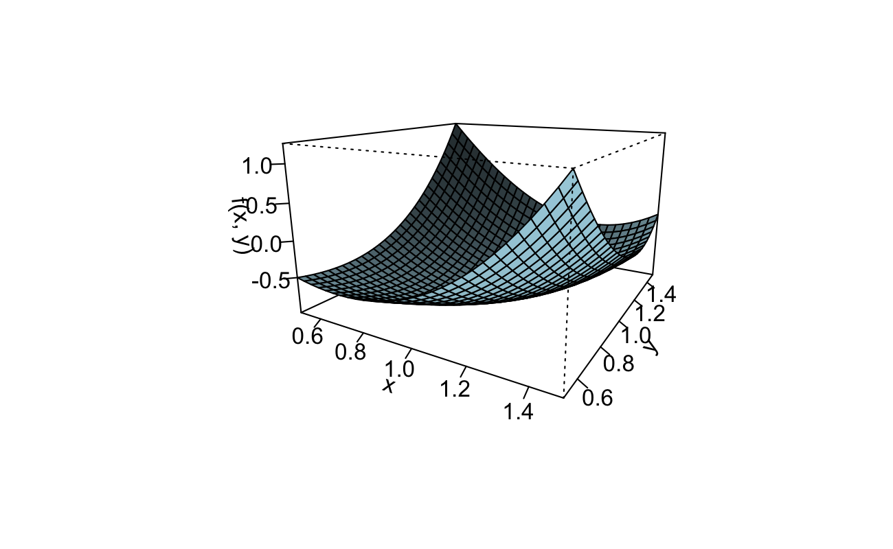
It looks like a little puddle could form if some rain fell on this surface.

9.5 Footnotes

https://en.wikipedia.org/wiki/Unit_circle ↩︎
https://en.wikipedia.org/wiki/Right_triangle ↩︎
The name for the longest side of a triangle↩︎
https://en.wikipedia.org/wiki/Pythagorean_trigonometric_identity ↩︎
https://en.wikipedia.org/wiki/Radian ↩︎
https://en.wikipedia.org/wiki/Inverse_function#Standard_inverse_functions ↩︎
Read Prof. R. Brown’s supplemental proof on this: https://math.jhu.edu/~brown/courses/f11/Concepts/Section3.3.pdf ↩︎
Note that it’s “bad form” to manipulate a string of equations on the left hand side, but I’m doing it anyway.↩︎
https://tutorial.math.lamar.edu/classes/calci/criticalpoints.aspx ↩︎
https://en.wikipedia.org/wiki/Gradient ↩︎
https://en.wikipedia.org/wiki/Saddle_point ↩︎
https://www.khanacademy.org/math/ap-calculus-ab/ab-diff-analytical-applications-new/ab-5-6b/a/concavity-review ↩︎
This idea of being able to “hold water” is a recurring theme for understanding the Saddlepoint Test, which we are leading up to.↩︎
https://en.wikipedia.org/wiki/Tuple ↩︎
This note requires you to remember some linear algebra: https://textbooks.math.gatech.edu/ila/determinants-volumes.html ↩︎
https://en.wikipedia.org/wiki/Hessian_matrix ↩︎
The determinant of a \(2x2\) matrix is \(ad - bc\). See https://www.cuemath.com/algebra/determinant-of-matrix/↩︎
There is some cool math/physics behind the geometry of this crisp shape: https://www.mechead.com/food-science-geometry-of-pringles/↩︎
https://en.wikipedia.org/wiki/Orthogonality ↩︎