# Thanks to ChatGPT for finding this package for me.
cquad::sq(J = 5, s = 2)
      [,1] [,2] [,3] [,4] [,5]
 [1,]    0    0    0    1    1
 [2,]    0    0    1    0    1
 [3,]    0    0    1    1    0
 [4,]    0    1    0    0    1
 [5,]    0    1    0    1    0
 [6,]    0    1    1    0    0
 [7,]    1    0    0    0    1
 [8,]    1    0    0    1    0
 [9,]    1    0    1    0    0
[10,] 1 1 0 0 02 The Binomial Distribution
2.1 Background
The binomial distribution extends the Bernoulli distribution to multiple trials. It models the number of successes in \((n)\) independent and identical Bernoulli experiments, each with probability of success \((p)\).
In other words, if we define \(Y = \sum\limits_{i=1}^{n}{X_i}\), where \(X_i \sim \text{Ber}(p)\), then \(Y \sim \text{Binom}(n,p)\)
2.1.1 Case Study: Binomial Distribution in Modern Policy
A recent example is COVID-19 vaccination coverage, modeled as the number of successes (vaccinated individuals) out of a fixed sample size.
For instance, a survey of 50 people in Miami-Dade County found 38 vaccinated. We model this as:
\[ X \sim \text{Binom}(n = 50, p) \]
Estimating \((p)\) helps public health policymakers monitor vaccination rates (Centers for Disease Control and Prevention 2022).
2.1.2 Current Uses in Biostatistics and Public Health
The binomial distribution is commonly used in biostatistics and public health, including
- Meta-analysis of disesase prevalance (Hamza, van Houwelingen, and Stijnen (2008), Nyaga, Arbyn, and Aerts (2014))
- Modeling presence/absence of gene families across microbial genomes (Snipen, Almøy, and Ussery (2009))
- Combining and estimating event rates (Young-Xu and Chan (2008))
- Modeling technical variation in scRNA-seq data (Sparta et al. (2024))
2.2 Deriving the Distribution
In the previous chapter, we explored the properties of a Bernoulli trial. We envisioned a scenario where a person flipped a coin five times, and the results were \(\{\)Heads, Tails, Heads, Tails, Tails\(\}\). What we knew, but the hypothetical person did no know, was that this particular coin was not “fair”. In fact, these five observations were drawn from a Bernoulli process with \(P[\text{Heads}] = 0.35\).
2.2.1 A Primer on Exchangeability
What if we saw \(\{\)Heads, Tails, Tails, Heads, Tails\(\}\) instead? The total number of heads and tails flipped is the same, but the order is different. Does that affect our estimate of \(p\)? In order to generalize this experiment a bit, we need to use the principle of exchangeability.1 The general idea of exchangeability is that the order of the observed flips doesn’t matter; i.e., that the coin doesn’t remember flipping a “Head” first then a “Tail”. Recall that we encoded the observed flips as \(\textbf{x} = (1,0,1,0,0)\). Therefore, if the order doesn’t matter, then all these rows will give us the same information about \(p\):
We see that there are 10 rows here, showing the 10 ways that we could flip \(| \textbf{x}| = 5\) coins sequentially and only see 2 heads2. While each of these rows shows the outcomes of different events, the resulting probability functions will be the same because of the commutative property of multiplication. That is, the likelihood function for the first row: \[ \prod\limits_{k = (0, 0, 0, 1, 1)} \left[ p^{k_i}(1 - p)^{1 - k_i} \right] = p^{\sum_k k_i}(1 - p)^{\sum_k (1 - k_i)} = p^2(1 - p)^3; \] yields the same polynomial as the likelihood function for the last row: \[ \prod\limits_{k = (1, 1, 0, 0, 0)} \left[ p^{k_i}(1 - p)^{1 - k_i} \right] = p^{\sum_k k_i}(1 - p)^{\sum_k (1 - k_i)} = p^2(1 - p)^3. \] The likelihood functions will be the same for all 10 rows.
2.2.2 The Binomial Coefficient
Let’s pretend that a prophet tells us that that the next time we flip \(n = 5\) coins we will see \(k = 2\) heads. We haven’t flipped any coins yet, but we have a vision of the future. If we encode 1 for heads and 0 for tails, we know that what is about to happen when we flip these 5 coins can be described by one of the 10 rows above. But how did we get there?
To make this process easier to explain, let’s flip 5 coins and leave them on the table, so that we can “see” our results as they happen. The 10 rows of the matrix above are based on the logic of this process:
- Before I flip any coins, there are \(n = 5\) coins in my hand. I haven’t flipped any coins yet, so all my options are available. There are 5 ways to flip one head.
- I flip the first coin, and after I set that coin aside, I have \(n - 1 = 4\) coins left for me to flip. There are still 4 ways to flip one head.
- I flip the second coin, and set it aside. I now have \(n - 2 = 3\) coins left to flip. There are 3 ways left to flip one head.
- I flip the third coin, and set it aside. Now things get interesting: I have \(n = k = 2\) coins left. If I have already flipped two heads in the first three flips, then I know the next two flips must be tails. If I haven’t flipped any heads in the first three flips, then I know the next two flips must be heads. If I’ve only flipped one head in the first three flips, then I know that one of the two next flips will be heads and the other will be tails (but I don’t know which is which).
- I flip the fourth coin and set it aside. The prophet already told me there would only be 2 heads in 5 flips, so the next flip is completely determined. If I have already flipped 2 heads with the first four coins, then this flip MUST be tails. If I’ve only flipped 1 head on the first four coins, then this flip MUST be heads. There is only one possible outcome, and it is predetermined to occur.
If we hadn’t been told by a prophet ahead of time that we would see two heads, then there would be \(n\) options for the first flip (I haven’t decided which coin to pick up yet, so that’s why I have 5 choices), \(n - 1\) for the second, all the way down to 1 way to flip at the end. That tells us there are \(n!\) ways these flips could have happened. There would have been \(5\times 4\times 3\times 2 = 120 = n!\) (this \(\\!\) symbol denotes the factorial3 of an integer) possible orderings and configurations of heads and tails. However, in our process, we’ve already assumed exchangeability, so the order of the flips does not matter. Not only that, but we are further limited: the prophet informed us that we MUST see exactly \(k = 2\) heads and \(n - k = 3\) tails. Because we use multiplication to “add” new possibilities, we must use division to take away these excluded possibilities. Since we must have \(k = 2\) heads, we remove 2 opportunities to flip tails; since we must have \(n - k = 3\) tails, we remove 3 opportunities to flip heads. Therefore, the number of options will be: \[ \frac{|\text{all results}|}{|\text{removed tails results}| \times |\text{removed heads results}|} = \frac{5!}{2!\times 3!} = \frac{120}{2 \times 6} = 10. \]
We then define the Binomial Coefficient as \[ {n \choose k} \equiv \frac{n!}{k!(n - k)!}. \]
2.2.3 Constructing the Distribution
To recap, we now have:
- a statement about the likelihood of a single binary event, of which \(k = 1\) denotes one class and \(k = 0\) denotes its complement (the other binary class): \(p^k(1 - p)^{1 - k}\),
- an experiment that yields a set of \(n\) such independent and exchangeable binary events, and
- a way to count all the ways that these events could possibly occur: \(\frac{n!}{k!(n - k)!}\).
Let us assume that the number of trials, \(n\), is known. We will now construct a probability function for the random variable \(k = 0, 1, \ldots, n\). We still assume independence and exchangeability, so the probability of success, \(p\), is fixed. Then, this function will first have a the binomial coefficient, then the probability to observe \(k\) successes, and finally the probability to observe \(n - k\) failures. Thus, the Binomial Distribution is:
\[ f(k|n,p) \equiv {n \choose k} p^{k}(1 - p)^{n - k}. \]
2.3 Example Random Samples
Code
set.seed(20150516)

N <- 10
bins_int <- seq.int(from = -1, to = N, by = 1)

xSymm <- rbinom(n = 100, size = N, prob = 0.5)
samplesSymm_ls <- list(
  n5   = xSymm[1:5],
  n15  = xSymm[1:15],
  n30  = xSymm[1:30],
  n100 = xSymm
)

xSkew <- rbinom(n = 100, size = N, prob = 0.2)
samplesSkew_ls <- list(
  n5   = xSkew[1:5],
  n15  = xSkew[1:15],
  n30  = xSkew[1:30],
  n100 = xSkew
)

rm(xSymm, xSkew)
Code
par(mfrow = c(2, 2))

hist(samplesSymm_ls$n5, breaks = bins_int)
hist(samplesSymm_ls$n15, breaks = bins_int)
hist(samplesSymm_ls$n30, breaks = bins_int)
hist(samplesSymm_ls$n100, breaks = bins_int)

par(mfrow = c(1, 1))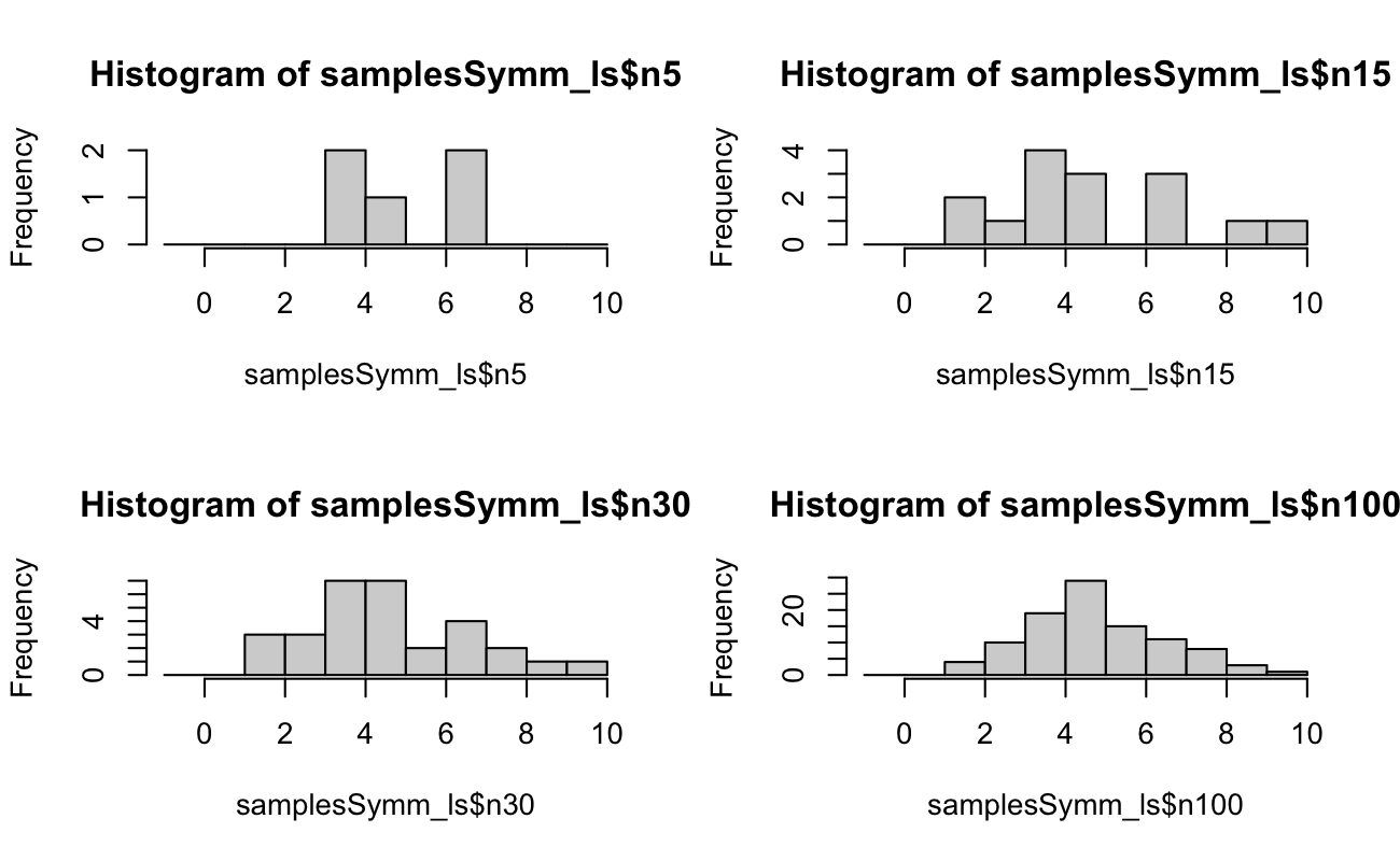
Code
par(mfrow = c(2, 2))

hist(samplesSkew_ls$n5, breaks = bins_int)
hist(samplesSkew_ls$n15, breaks = bins_int)
hist(samplesSkew_ls$n30, breaks = bins_int)
hist(samplesSkew_ls$n100, breaks = bins_int)

par(mfrow = c(1, 1))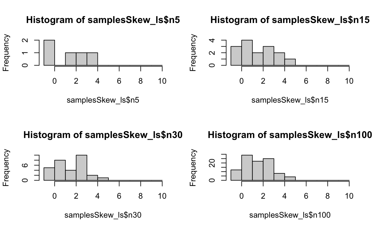
2.4 Example with Data: Vaccine Trial Outcomes
Suppose researchers conduct a clinical trial of a new vaccine. Each participant either develops immunity (success) or does not (failure). If \((n = 20)\) participants are tested, and each has probability \((p = 0.7)\) of developing immunity, then the number of immune participants, \((X)\), follows a binomial distribution:
\[ X \sim \text{Binom}(n = 20, p = 0.7) \]
The probability of observing exactly 15 immune participants is:
\[ P(X = 15) = \binom{20}{15}(0.7)^{15}(0.3)^5 \]
This example highlights how the binomial distribution models real-world binary outcomes in public health and medical research. It captures the distribution of the number of “successes” across repeated independent trials, which is fundamental for evaluating treatments, surveys, and risk assessments.
2.5 Formal Foundations
2.5.1 Pascal’s Rule
For writing proofs involving combinations, we need the following property, known as Pascal’s Formula,4 which states that
\[ {a \choose b} = {a - 1 \choose b} + {a - 1 \choose b - 1}. \]
Proof: For integers \(a,b\), we construct this identity directly via simplification: \[ \begin{aligned} {a - 1 \choose b} + {a - 1 \choose b - 1} &= \frac{(a - 1)!}{b!(a - b - 1)!} + \frac{(a - 1)!}{(b - 1)!(a - 1 - b + 1)!} \\ &= \frac{a - b}{a - b}\left[ \frac{(a - 1)!}{b!(a - b - 1)!} \right] + \frac{b}{b} \left[ \frac{(a - 1)!}{(b - 1)!(a - b)!} \right] \\ &= \frac{a(a - 1)! - b(a - 1)!}{b!(a - b)(a - b - 1)!} + \frac{b(a - 1)!}{b(b - 1)!(a - b)!} \\ &= \frac{a! - b(a - 1)!}{b!(a - b)!} + \frac{b(a - 1)!}{b!(a - b)!} \\ &= \frac{a!}{b!(a - b)!} \\ &\equiv {a \choose b}. \end{aligned} \]
2.5.2 Mathematical Induction
The next foundational proof requires a technique called “Proof by Induction”, or more generally, mathematical induction.5 This is the structure of such a proof:
Proof by Induction: Consider a sequence of equations indexed over the integers by \(n\). To show that the sequence of equations is true \(\forall n\), we
- show that the equation is true for \(n = 1\) [the “base case”],
- assume that the equation is true for \(n = i\) [the “hypothesis”], then
- prove that the equation is true for \(n = i + 1\) from the case when \(n = i\) [the “induction”].
Here is a trivial example. Let’s prove \(\forall k \in\mathbb{N} \ge 5\) that \(2^k < \Gamma(k + 1)\) (the point of this proof is to show that the factorial function increases more rapidly to \(\infty\) than the exponential function). Our base case is for \(k = 5\). We know that \(2^5 = 32\) and \(\Gamma(k + 1) = k! = 5! = 120\). Because \(32 < 120\), the base case is true. Our hypothesis, what we assume to be true, is that \(2^i < \Gamma(i + 1)\). To logically induct, we assume our hypothesis is true, and then show that our hypothesis implies that \(2^{i + 1} < \Gamma(i + 2)\). That is \[ \begin{aligned} 2^{i+1} &\overset{?}{<} \Gamma(i + 2) \\ \Longrightarrow 2 \times 2^i &\overset{?}{<} i \times \Gamma(i + 1) \\ \Longrightarrow \frac{2}{i} \times 2^i &< \Gamma(i + 1), \end{aligned} \] which is true for \(i \ge 5\) because our hypothesis was that \(2^i < \Gamma(i + 1)\). Thus, \(2^k < \Gamma(k + 1)\ \forall k \in\mathbb{N} \ge 5\), which completes our proof.
2.5.3 Mathematical Induction Proof of the Binomial Theorem
For this section, we will also need to use the Binomial Theorem:6
\[ (x + y)^n = \sum_{k = 0}^n {n \choose k} x^k y^{n - k}. \]
Before we can use this, we must prove that it is true.
2.5.3.1 The Base Case
Let \(n = 1\). Then
\[ \begin{aligned} \sum_{k = 0}^1 {1 \choose k} x^k y^{1 - k} &= \left[ {1 \choose 0} x^0 y^{1 - 0} \right] + \left[ {1 \choose 1} x^1 y^{1 - 1} \right] \\ &= \frac{1!}{0!\times 1!} (1) y^1 + \frac{1!}{1!\times 0!} x^1(1) \\ &= y + x \\ &= (x + y)^1. \end{aligned} \]
2.5.3.2 The Hypothesis
We assume that this equation is true for \(n = i\). That is, we assume that
\[ \sum_{k = 0}^i {i \choose k} x^k y^{i - k} = (x + y)^i. \]
2.5.3.3 The Induction
Assuming that the hypothesis for \(n = i\) is true, we will show that the equation also holds for \(n = i + 1\). Note that the end of the proof requires Pascal’s Rule to combine sums of combinations, and we comment that there is only one way to “choose” 0 things or all things. Thus,
\[ \begin{aligned} (x + y)^i &= \sum_{k = 0}^i {i \choose k} x^k y^{i - k} \\ \Longrightarrow (x + y)^{i + 1} &= (x + y)\sum_{k = 0}^i {i \choose k} x^k y^{i - k} \\ &= (x + y)\left[ {i \choose 0} x^0 y^{i - 0} + {i \choose 1} x^1 y^{i - 1} + \ldots + {i \choose i - 1} x^{i - 1} y^1 + {i \choose i} x^{i - 0} y^0 \right] \\ &= x\left[ {i \choose 0} x^0 y^i + {i \choose 1} x^1 y^{i - 1} + \ldots + {i \choose i - 1} x^{i - 1} y^1 + {i \choose i} x^i y^0 \right] + \\ &\quad\ \ y\left[ {i \choose 0} x^0 y^i + {i \choose 1} x^1 y^{i - 1} + \ldots + {i \choose i - 1} x^{i - 1} y^1 + {i \choose i} x^i y^0 \right] \\ &= \left[ {i \choose 0} x^1 y^i + {i \choose 1} x^2 y^{i - 1} + \ldots + {i \choose i - 1} x^i y^1 + {i \choose i} x^{i+1} y^0 \right] + \\ &\quad\ \left[ {i \choose 0} x^0 y^{i + 1} + {i \choose 1} x^1 y^i + \ldots + {i \choose i - 1} x^{i - 1} y^2 + {i \choose i} x^i y^1 \right] \\ \\[0.1mm] &\qquad \text{\emph{Collect like terms...}} \\ &= {i \choose 0} x^0 y^{i + 1} + \\ &\qquad \left[ {i \choose 0} x^1 y^i + {i \choose 1} x^1 y^i\right] + \ldots + \left[ {i \choose i - 1} x^i y^1 + {i \choose i} x^i y^1 \right] + \\ &\qquad {i \choose i} x^{i+1} y^0 \\ \\[0.1mm] &\qquad \text{\emph{Only one way to choose all or none...}} \\ &= (1) x^0 y^{i + 1} + \\ &\qquad \left[ {i \choose 0} + {i \choose 1} \right]x^1 y^i + \ldots + \left[ {i \choose i - 1} + {i \choose i} \right]x^i y^1 + \\ &\qquad (1) x^{i+1} y^0 \\ \\[0.1mm] &\qquad \text{\emph{Pascal's Rule...}} \\ &= (1) x^0 y^{i + 1} + \\ &\qquad \left[ {i + 1 \choose 1} \right]x^1 y^i + \ldots + \left[ {i + 1 \choose i} \right]x^i y^1 + \\ &\qquad (1) x^{i+1} y^0 \\ &= {i + 1 \choose 0} x^0 y^{i + 1} + {i + 1 \choose 1}x^1 y^i + \ldots + {i + 1 \choose i}x^i y^1 + {i + 1 \choose i + 1} x^{i+1} y^0 \\ \\[0.1mm] &\qquad \text{\emph{By definition...}} \\ &= \sum_{k = 0}^{i + 1} {i + 1 \choose k} x^k y^{i + 1 - k}. \end{aligned} \]
Therefore, \(\forall n \in \mathbb{N}\), \[ \sum_{k = 0}^n {n \choose k} x^k y^{n - k} = (x + y)^n. \]
2.6 Show that this is a Distribution
Let \(\mathcal{S} = \mathbb{N} \cup 0\), where \(\mathbb{N}\) denotes the set of natural numbers.7 Let \(f(k|n,p) = {n \choose k} p^{k}(1 - p)^{n - k}\) represent the probability function of the Binomial Distribution. We must now show that
- \(\forall k \in \mathcal{S}\), and for \(p \in (0,1)\), \(f(k|n, p) \ge 0\), and
- for \(p \in (0,1)\), \(\int_{k \in \mathcal{S}} \text{d}F(k|n,p) = 1\).
2.6.1 The Distribution is Non-negative
Consider \(f\) defined above. First, we notice that the Binomial Coefficient is defined as a ratio of factorials; the standard definition of factorials only includes the natural numbers (\(\mathbb{N}\)), so they are necessarily positive. The ratio of two positive numbers is positive. Second, we have that \(k,\ n - k \ge 0\), and that \(p > 0\). Non-negative powers of positive numbers are also positive. Setting \(p = 0\) yields a degenerate distribution anyway, so we don’t bother with it. Putting these together for \(p \in (0,1)\), we have that \(f = 0\) outside the support of \(k\) and \(f > 0\) for \(k \le n, \ni \{k,\ n\} \in \mathcal{S}\).
2.6.2 The Total Probability is 1
Recall the Binomial Theorem we proved above, and let \(x = p\) and \(y = 1 - p\). Then, \[ \begin{aligned} \int_{k \in \mathcal{S}} \text{d}F(k|n,p) &= \sum_{k = 0}^n {n \choose k} p^{k}(1 - p)^{n - k} \\ &= \left[ p + (1 - p) \right]^n \\ &= 1^n \\ &= 1. \end{aligned} \]
Therefore, because the function \(f(k|n,p)\) is always non-negative and it’s Riemann-Stieljes integral is 1, the Binomial Distribution is a true distribution.
2.7 Derive the Moment Generating Function
Deriving the MGF for the Binomial is a straightforward application of the definition and Binomial Theorem. That is, \[ \begin{aligned} M_k(t) &\equiv \mathbb{E}\left[ e^{tX} \right] \\ &= \int\limits_{k \in \mathcal{S}(K)} e^{tk} \text{d}F_K(k|n,p) \\ &= \sum\limits_{k = 0}^n e^{tk} {n \choose k} p^{k}(1 - p)^{n - k} \\ &= \sum\limits_{k = 0}^n {n \choose k} \left[e^t\right]^k p^{k}(1 - p)^{n - k} \\ &= \sum\limits_{k = 0}^n {n \choose k} \left[e^tp\right]^k (1 - p)^{n - k} \\ &= \left[ e^tp + (1 - p) \right]^n. \end{aligned} \]
2.8 Method of Moments Estimators
Now that we have this MGF, we can find the Method of Moments (MoM) estimator for \(p\), and we will comment on such an estimator for \(n\) when it is unknown.
2.8.1 The First Moment
We have that \[ \begin{aligned} M_k(t) &= \left[ e^tp + (1 - p) \right]^n \\ \Longrightarrow M^{\prime}_k(t) &= \frac{\partial}{\partial t} \left[ e^tp + (1 - p) \right]^n \\ &= n \left[ e^tp + (1 - p) \right]^{n - 1} \frac{\partial}{\partial t} \left[ e^tp + (1 - p) \right] \\ &= n \left[ e^tp + (1 - p) \right]^{n - 1} e^tp \\ \Longrightarrow M^{\prime}_k(0) &= n \left[ (1)p + (1 - p) \right]^{n - 1} (1)p \\ &= n(1)^{n - 1}p \\ &= np. \end{aligned} \] Therefore, \(\mathbb{E}[k] = np\).
2.8.2 The Second Non-Central Moment
Taking the second derivative with respect to \(t\), we have \[ \begin{aligned} M^{\prime}_k(t) &= ne^tp \left[ e^tp + (1 - p) \right]^{n - 1} \\ \Longrightarrow M^{\prime\prime}_k(t) &= ne^tp \frac{\partial}{\partial t} \left[ e^tp + (1 - p) \right]^{n - 1} + \left[ e^tp + (1 - p) \right]^{n - 1} \frac{\partial}{\partial t} ne^tp \\ &= ne^tp \times (n - 1) \left[ e^tp + (1 - p) \right]^{n - 2} e^tp + \left[ e^tp + (1 - p) \right]^{n - 1} ne^tp \\ \Longrightarrow M^{\prime\prime}_k(0) &= n(1)p \times (n - 1) \left[ (1)p + (1 - p) \right]^{n - 2} (1)p + \left[ (1)p + (1 - p) \right]^{n - 1} n(1)p \\ &= np^2 (n - 1) (1)^{n - 2} + np (1)^{n - 1} \\ &= np \left[(n - 1)p + 1\right]. \end{aligned} \] Therefore, \(\mathbb{E}[k^2] = np(np - p + 1)\).
2.8.3 The Second Central Moment
Thus \[ \begin{aligned} \text{Var}[k] &= \mathbb{E}[k^2] - \left(\mathbb{E}[k]\right)^2 \\ &= np(np - p + 1) - \left( np \right)^2 \\ &= np \left[ np - p + 1 - np \right] \\ &= np (1 - p). \end{aligned} \]
Technically, we don’t need the second central moment for this distribution to find the Method of Moments estimators, but it is good practice.
2.8.4 Solving the System of Equations
Now that we have the first two population moments, \(\mathbb{E}[k]\) and \(\text{Var}[k]\), we can set them equal to the first two sample moments. That is, we solve the system \[ \left\{ \mathbb{E}[k] = \frac{1}{N} \sum_{i = 1}^N k_i;\ \mathbb{E}[k^2] = \frac{1}{N} \sum_{i = 1}^N k_i^2 \right\}, \] where \(N\) is the number of Binomial experiments and \(k_i\) is the number of successes out of \(n\) attempts in Binomial experiment \(i\). For our example data, we were discussing the first such experiment, with observed data \(\{\)Heads, Tails, Heads, Tails, Tails\(\}\); so we are on Binomial experiment \(i\), the number of coin flips was \(n = 5\), and we observed \(k_i = 2\) heads.
Given repeated \(N\) Binomial experiments of \(n\) Bernoulli trials each, we then solve the following system of equations: \[ \left\{ np = \frac{1}{N} \sum_{i = 1}^N k_i;\ np(np - p + 1) = \frac{1}{N} \sum_{i = 1}^N k_i^2 \right\}. \] Very often, \(n\) is known, so this simplifies to solving \(\hat{p}_{MoM} = \frac{1}{nN} \sum_{i = 1}^N k_i\).
2.9 Method of Moments Estimates from Observed Data
Recall our “observed” data: \(\{\)Heads, Tails, Heads, Tails, Tails\(\}\). This was an observation from 5 independent Bernoulli trials or only ONE Binomial experiment with \(n = 5\) and \(k = 2\). We need more than \(N = 1\) if we want to estimate moments! If you remember the introduction, we generated this data from a Bernoulli process with \(p = 0.35\). Let’s generate some more samples, this time we will have \(N = 7\) experiments where we flipped \(n = 5\) coins each time, with the same probability of success \(p = 0.35\) as before:
Code
# Reset our seed
set.seed(20150516)

# Generate our sample
observed_int <- rbinom(
  n = 7,      # number of Binomial experiments, N
  size = 5,   # number of Bernoulli Trials per experiment, n
  prob = 0.35 # probability of success for each Bernoulli Trial
)

# Inspect
observed_int
[1] 3 1 2 3 1 0 1
For these \(N\) = 7 Binomial trials (each with \(n = 5\) flips), we observed the following number of heads: 3, 1, 2, 3, 1, 0, 1.
2.9.1 Case When \(n\) is Known
This is the most common case. Recall that we need the averages of \(k_i\) and \(k_i^2\), so let’s calculate these first.
Code
k_df <-
  tibble(k = observed_int) %>%
  mutate(k2 = k^2)
k_df
# A tibble: 7 × 2
      k    k2
  <int> <dbl>
1     3     9
2     1     1
3     2     4
4     3     9
5     1     1
6     0     0
7     1     1

kBar_num <- colMeans(k_df)
kBar_num
   k   k2
1.57 3.57
So, \(\frac{1}{7} \sum_i k_i\) = 1.5714286 and \(\frac{1}{7} \sum_i k_i^2\) = 3.5714286. Thus, the two equations in our system are
- \(np\) = 1.571
- \(np(np - p + 1)\) = 3.571
However, we already said that \(n = 5\) is known, so we don’t need the second equation. All we have to solve is \(np = (5)p = 1.571 \Rightarrow \hat{p}_{MoM} = 0.314\).
2.9.1.1 Case When \(n\) is Unknown
This is a rare case, and usually only a theoretical exercise, though it can happen in ecological studies of species. One example could be where a park ranger goes deep into the woods on 5 different days. While on patrol, they encounter one grey wolf on the first day, none on the second, one on the third, and none on the fourth and fifth. In this case, we still have \(|\text{Count of observed wolves}| = |\textbf{x}| = \{1, 0, 1, 0, 0\}\). In this case, we don’t actually know how many grey wolves are in the park close enough to the ranger to even be detected. Thus, we could think about this as 5 Binomial trials with unknown \(n\).
Now, we have the same system as above, but it is no longer trivial. We know that the ranger went out on \(N = 5\) days, and we know that \(\sum_i k_i = \sum_i k_i^2 = 2\). So, by simplifying the first equation, we have that: \[ \begin{aligned} np &= \frac{1}{N}\sum_i k_i \\ \Longrightarrow np &= \frac{1}{5}(2) \\ \Longrightarrow np &= 0.4\\ \Longrightarrow p &= \frac{0.4}{n}. \end{aligned} \]
We substitute these known quantities into the second equation: \[ \begin{aligned} np(np - p + 1) &= \frac{1}{N}\sum_i k_i^2\\ \Longrightarrow \left( 0.4 \right) \left(\left[ 0.4 \right] - \left[ \frac{0.4}{n} \right] + 1\right) &= \frac{1}{5}(2) \\ \Longrightarrow \left(0.4 - \frac{0.4}{n} + 1\right) &= 1 \\ \Longrightarrow 0.4 - \frac{0.4}{n} &= 0 \\ \Longrightarrow 0.4 &= \frac{0.4}{n} \\ \Longrightarrow n &= 1, \end{aligned} \] which is clearly an underestimate for \(n\)! Because, when we substitute this estimate back in to solve for \(p\), we get \(p = 0.4\), we should be very suspicious that only one wolf lives in the entire forest. I recommend that students read the primer from DasGupta and Rubin (2004) at this juncture.
2.10 Maximum Likelihood Estimators
2.10.1 The Likelihood Function
Let’s continue our example of 7 Binomial trials with 5 flips each during which we observed \(\textbf{k}\) = 3, 1, 2, 3, 1, 0, 1 heads. In this case, we know that \(n = 5\) and \(N = 7\), so the Likelihood of \(p\) given \(\textbf{k}\) is \[ \begin{aligned} \mathcal{L}(p|\textbf{k}, n) &= \prod\limits_{i = 1}^{N = 7} {n \choose k_i} p^{k_i} (1 - p)^{n - k_i} \\ &= \left[ {5 \choose 3} p^3 (1 - p)^{5 - 3} \right] \times \left[ {5 \choose 1} p^1 (1 - p)^{5 - 1} \right] \times \left[ {5 \choose 2} p^2 (1 - p)^{5 - 2} \right] \times \left[ {5 \choose 3} p^3 (1 - p)^{5 - 3} \right] \times \\ &\qquad \left[ {5 \choose 1} p^1 (1 - p)^{5 - 1} \right] \times \left[ {5 \choose 0} p^0 (1 - p)^{5 - 0} \right] \times \left[ {5 \choose 1} p^1 (1 - p)^{5 - 1} \right] \\ &= {5 \choose 3}{5 \choose 1}{5 \choose 2}{5 \choose 3}{5 \choose 1}{5 \choose 0}{5 \choose 1} p^{11} (1 - p)^{7\times 5 - 11}. \end{aligned} \]
Note that all the Binomial Coefficient terms in the beginning are just multiplicative constants. The real “action” is happening in the \(p^{11}(1 - p)^{35 - 11}\) part; this is known as the kernel8 of the likelihood. How do we know this? Because \(x\)-value locations of the the extreme values of \(cf(x)\) are the same as the \(x\)-value locations for the extreme values of \(f(x)\).
Proof: Let \(f\) be a differentiable function with \(M\) extreme values given by \(\{(x_1, f(x_1)), (x_2, f(x_2)), \ldots, (x_M, f(x_M))\}\). Therefore, for \(i = 1, 2, \ldots, M\), \(f^{\prime}(x_i) = 0\). Therefore, for any constant \(c < \infty\), \(cf^{\prime}(x_i) = 0\). Hence, the extreme values of \(cf(x)\) are \(\{(x_1, cf(x_1)), (x_2, cf(x_2)), \ldots, (x_M, cf(x_M))\}\).
Therefore, it is commonplace to write the likelihood as a proportional relationship, \[ \mathcal{L}(p|\textbf{k}, n) \propto p^{11} (1 - p)^{24}, \] where \(\propto\) is read “is proportional to”.
This kernel function is of incredible importance: \(\mathcal{L}\) contains almost all the information known about \(p\). It has all the data and it also has our best guess of the data generating process (a Binomial process in this case). However, we note that \(\mathcal{L}\) is not a probability distribution of \(p\). If it was, then we could make probabalistic statements about the values of \(p\) which generated the observed data \(\textbf{k}\).
2.10.2 A Probability Function of \(p\)
How can I so sure that \(\mathcal{L}\) is not a probability distribution? It’s clearly non-negative, so let’s find out what it integrates to. That is, \[ \begin{aligned} \int_0^1 \mathcal{L}(p|\textbf{k},n)dp &= \int_0^1 {5 \choose 3}{5 \choose 1}{5 \choose 2}{5 \choose 3}{5 \choose 1}{5 \choose 0}{5 \choose 1} p^{11} (1 - p)^{24}dp \\ &= C(5, \textbf{k}) \int_0^1 p^{11} (1 - p)^{24} dp, \end{aligned} \] where \(C(5, \textbf{k})\) is the constant product of the seven Binomial Coefficients. Further, while we have not yet derived this distribution, for \(x \in (0,1)\), \(x^A(1 - x)^B\) is the kernel of a Beta distribution with \(A = \alpha - 1\) and \(B = \beta - 1\). That is \[ f_{\text{Beta}}(p|\alpha,\beta) \equiv \frac{\Gamma(\alpha + \beta)}{\Gamma(\alpha)\Gamma(\beta)} p^{\alpha - 1}(1 - p)^{\beta - 1}. \] Since the Beta distribution is a statistical distribution, we know that its integral over \((0,1)\) is equal to 1. Therefore, \[ \begin{aligned} \int_0^1 \mathcal{L}(p|\textbf{k},n)dp &= C(5, \textbf{k}) \int_0^1 p^{12 - 1} (1 - p)^{25 - 1} dp \\ &= C(5, \textbf{k}) \int_0^1 \frac{\Gamma(12)\Gamma(25)}{\Gamma(12 + 25)} \frac{\Gamma(12 + 25)}{\Gamma(12)\Gamma(25)} p^{12 - 1} (1 - p)^{25 - 1} dp \\ &= C(5, \textbf{k}) \frac{\Gamma(12)\Gamma(25)}{\Gamma(12 + 25)} \int_0^1 f_{\text{Beta}}(p|\alpha = 12,\beta = 25) dp \\ &= C(5, \textbf{k}) \frac{\Gamma(12)\Gamma(25)}{\Gamma(12 + 25)}, \end{aligned} \] which is clearly not equal to 1. But, this effort is not in vain, because it yields the multiplicative constant that makes \(\mathcal{L}\) into a probability function of \(p\). That is, \[ \begin{aligned} f(p|\textbf{k}, n = 5) &= \frac{1}{C(5, \textbf{k})} \frac{\Gamma(12 + 25)}{\Gamma(12)\Gamma(25)} \mathcal{L}(p|\textbf{k},n = 5) \\ &= \frac{1}{C(5, \textbf{k})} \frac{\Gamma(12 + 25)}{\Gamma(12)\Gamma(25)} C(5, \textbf{k}) p^{12 - 1} (1 - p)^{25 - 1} \\ &= \frac{\Gamma(12 + 25)}{\Gamma(12)\Gamma(25)} p^{12 - 1} (1 - p)^{25 - 1} \\ &= f_{\text{Beta}}(p|\alpha = 12,\beta = 25). \end{aligned} \] We can use this distribution to estimate the probability that \(p\) is fair. For example, a fair coin with the same total number of flips (35) would have a Beta distribution with \(\alpha = \beta = (35 + 2)/2 = 18.5\). Under such a distribution, the probability that \(p \in (0.4, 0,6)\) is calculated by:
Code
pbeta(q = 0.6, shape1 = 18.5, shape2 = 18.5) -
  pbeta(q = 0.4, shape1 = 18.5, shape2 = 18.5)
[1] 0.778
That is, if we had observed balanced data with the same sample sizes, then \(\mathbb{P}[0.4 < p < 0.6] = 0.778\). However, what we actually observed was that
Code
pbeta(q = 0.6, shape1 = 12, shape2 = 25) -
  pbeta(q = 0.4, shape1 = 12, shape2 = 25)
[1] 0.162
Thus, given the data we actually observed, \(\mathbb{P}[0.4 < p < 0.6] = 0.162\). In terms of pure probability, this statement can be interpreted as “given the data we observed, there is a 16% chance that the coin is fair”.
2.10.3 Estimating the Most “Likely” Value
While being able to describe the probability that the coin is “fair” is valuable, we often are interested in answering the question “what is the most likely value of \(p\) given the data we observed?” Now we are finally discussing maximum likelihood estimation. Given the data we observed, what value of \(p\) makes \(\mathcal{L}\) attain its maximum value? We find a candidate value as follows: \[ \begin{aligned} \mathcal{L}(p|\textbf{k},n) &= C(5, \textbf{k}) p^{11} (1 - p)^{24} \\ \Longrightarrow \ell(p|\textbf{k},n) &= \log \left[ C(5, \textbf{k}) \right] + 11\log p + 24\log(1 - p) \\ \Longrightarrow \frac{\partial}{\partial p} \ell(p|\textbf{k},n) &= 0 + \frac{11}{p} + \frac{24}{1 - p}(-1) \\ &= \frac{11}{p} - \frac{24}{1 - p} \\ \Longrightarrow 0 &\overset{set}{=} \frac{11}{\hat{p}} - \frac{24}{1 - \hat{p}} \\ &= 11(1 - \hat{p}) - 24\hat{p} \\ &= 11 - 35\hat{p} \\ \Longrightarrow \hat{p}_{MLE} &= \frac{11}{35} \approx 0.314. \end{aligned} \] So we know that \(\mathcal{L}\) attains an extreme value at \(\hat{p}_{MLE} = 0.314\), but is it a maximum? We check this using the second derivative test: \[ \begin{aligned} \frac{\partial}{\partial p} \ell(p|\textbf{k},n) &= \frac{11}{p} - \frac{24}{1 - p} \\ \Longrightarrow \frac{\partial^2}{\partial p^2} \ell(p|\textbf{k},n) &= -\frac{11}{p^2} - (-1)\frac{24}{(1 - p)^2}(-1) \\ &= -\left( \frac{11}{p^2} + \frac{24}{(1 - p)^2} \right) \\ &< 0. \end{aligned} \] Therefore, \(\hat{p}_{MLE} = 0.314\) is the Maximum Likelihood Estimator for \(p\).
2.11 Exercises
Show that the Binomial distribution can be approximated by the Poisson distribution as \(n \rightarrow \infty\)
Using the dataset below:
- Use the method of moments to estimate \((p)\) for Community A.
- Calculate the maximum likelihood estimator (MLE) for \((p)\).
- Compare the two estimators.
- Use the method of moments to estimate \((p)\) for Community A.
| Community | Vaccinated | Sample Size |
|---|---|---|
| A | 38 | 50 |
| B | 42 | 60 |
| C | 55 | 70 |
Titanicsurvival data is a 4-way contingency table built from the British Board of Trade (1912) inquiry counts and used to model the Binomial distribution. The data is built into base R and also available as a row-level CSV on Kaggle. Each passenger is a unique Bernoulli trial, and fixing a group of n passengers makes the total number of survivors K follow a Binomial(n, p) distribution. TheTitanicdataset contains 2,201 individual records with 3 binary categorical variables: Sex (male/female), Age (child/adult), and Survived (no/yes). Using this dataset:- Plot the distributions of the 3 binary variables
Sex,Age, andSurvived - Calculate the method of moments estimator for \(p\) for the variable
Survived - Calculate the maximum likelihood estimator for \(p\) for the variable
Survived - Compare the two estimators.
- Plot the distributions of the 3 binary variables
Show that the sum of \(n\) Bernoulli distributed random variables follows a Binomial(n,p) distribution.
Suppose \(X \sim \text{Binom}(n, p)\) but both \((n)\) and \(p\) are unknown. Describe the process you would take to estimate \(n\). What are the challenges to estimate this parameter if it were truly unknown?
2.12 Footnotes
Read all the pages of this short lesson, as it also includes a refresher on Riemann-Stieltjes Integrals: https://www.colorado.edu/amath/sites/default/files/attached-files/definetti.pdf↩︎
The symbol \(|\cdot|\) represents the cardinality operator: https://en.wikipedia.org/wiki/Cardinality↩︎
See the “Bayesian Statistics” section of the article on statistical kernels: https://en.wikipedia.org/wiki/Kernel_(statistics)↩︎