The Normal Distribution (also called the Gaussian Distribution after Carl Friedrich Gauss1) is first and foremost the “mistakes” distribution. Gauss derived this distribution to explain the discrepencies between multiple junior (or even senior) astronomers’ reported planetary positions. As a quick note, this derivation is absolutely monstrous (Gauss’ genius was orders of magnitude beyond my intelligence). We will follow the general premise of Prof. Xi Chen’s translation and understanding of Gauss’ original notes (and Prof. Chen’s comprehensive understanding of the history of mathematics and statistics); he published his thoughts in his blog “Not a Rocket Scientist” in his 27 January 2023 post.
10.1.1 Preliminary Notation and Assumptions
We begin by noting that if we have only one measurement, that single measurement is our best guess for the truth. Let’s denote it \(m\). Also, we assume that:
If we add more independent measurements, we can use the arithmetic mean to “summarize” them well.
If we add more independent measurements from similarly trained astronomers, these new values can be described positive or negative deviations (i.e., mistakes or errors) from the first measurement.
These mistakes/deviations/errors should be independently and symmetrically distributed around 0
by random chance, an astronomer is just as likely to write down a number slightly smaller than the “truth” as they would be to write down a slightly larger number; and,
these astronomers are all similarly trained and trying their best, so we expect the mistake distribution to be the same for all astronomers.
Smaller mistakes/deviations/errors are more likely to occur than larger errors.
“It has been customary to regard as an axiom the hypothesis that if any quantity has been determined by several direct observations, made under the same circumstances and with equal care, the arithmetic mean of the observed values will yield the most probable value…
We start by assuming that the first measurement is the correct one (which is obviously wrong, but it allows us to understand what’s happening, and the assumption will be quickly discarded). If we have \(n\) independent attempts to measure the same true value (like the angle of one planet relative to another), denoted \(X_1, X_2, \ldots, X_n\), the mistake (error) components of these measures can be defined as \[
[E_1, E_2, \ldots, E_n] = [X_1, X_2, \ldots, X_n] - m.
\]
10.1.2 Applying Assumptions
As we assumed above, these mistakes are all independent and identically distributed according to some distribution. We denote this as \[
E_i \overset{iid}{\sim} f_E(\varepsilon).
\] As we already assumed, errors are symmetric around 0. Thus, we know that \(f_E(\varepsilon) = f_E(-\varepsilon)\). Further, because we also assume that errors near 0 are more likely than errors further away, this leads us to create a likelihood function. While, we do have a vector of observed data (the errors, \(E_i\)), we don’t know what kinds of parameter space we are optimizing over. So, we will present the general form of some likelihood function optimization with an unspecified parameter suite (the empty dot): \[
\begin{aligned}
\mathcal{L}(\circ|\textbf{E}) &= \prod_{i = 1}^n f(\varepsilon_i|\circ) \\
\Longrightarrow \ell(\circ|\textbf{E}) &= \sum_{i = 1}^n \log\left[ f(\varepsilon_i|\circ) \right] \\
\Longrightarrow \frac{\partial}{\partial\circ} \ell(\circ|\textbf{E}) &= \sum_{i = 1}^n \frac{f^{\prime}(\varepsilon_i|\circ)}{f(\varepsilon_i|\circ)}.
\end{aligned}
\]
Now we have to take a step back here. We have no idea what \(f\) looks like, so we have no idea what \(\ell\) looks like, and we certainly have no idea to take a derivative with respect to some unknown group of parameters (we don’t even know how many there are), or even if we are taking the derivative with respect to the parameters at all! All we know is that we are taking the derivative of some function \(\ell\) with respect to something, and that we are treating the data as fixed so that we can find the functions \(\ell\) and \(f\) which fit the data best.
To make the notation a touch easier, let \(g_E(\varepsilon) = f^{\prime}(\varepsilon_i) / f(\varepsilon_i)\). Now, let’s apply some of Gauss’ intuition, that the arithmetic mean would be a good approximation of the truth; that is, Gauss assumed that \(\bar{X} \approx m\). Thus, \[
\begin{aligned}
\frac{\partial}{\partial\circ} \ell(\circ|\textbf{E}) &= \sum_{i = 1}^n \frac{f^{\prime}(\varepsilon_i|\circ)}{f(\varepsilon_i|\circ)} \\
&\qquad\text{\emph{Easier notation...}} \\
&= \sum_{i = 1}^n g_E(\varepsilon) \\
&\qquad\text{\emph{By definition...}} \\
&= \sum_{i = 1}^n g_E(X_i - m) \\
&\qquad\text{\emph{Gauss' intuition...}} \\
&\approx \sum_{i = 1}^n g_E(X_i - \bar{X}) \\
&\qquad\text{\emph{Assumption that mistakes centre around 0...}} \\
&= 0.
\end{aligned}
\] This may look trivial (obviously the sum of mistakes which centre at 0 should be approximately 0), but it allows us to make more clarifying statements about the original error function. Now, we have that we are looking for some \(f(\textbf{E}|\boldsymbol\theta) \ni \nabla\ell(\boldsymbol\theta|\textbf{E}) = \textbf{0}\)2. Notice that this relationship will hold for any properly constructed sample \(\textbf{X}\), because we are constructing\(f\) to have this property.
10.1.3 Clues About \(g_E\)
We are being good little detectives so far. We know a couple things now: \[
\begin{aligned}
\nabla \ell(\boldsymbol\theta|\textbf{E}) \approx \sum_{i = 1}^n g_E(X_i - \bar{X}) &= 0 \\
\sum_{i = 1}^n x_i - n\bar{x} &= 0.
\end{aligned}
\] The first is what we discovered last section. The second is by definition. So we need a family of functions for \(g_E\) so that \[
\sum_{i = 1}^n g_E(X_i - \bar{X}) = \sum_{i = 1}^n X_i - n\bar{X}.
\] So, we need a function \(g_E\) that will allow the summation operator to “pass through”, so that \[
\sum_{i = 1}^n g_E(X_i - \bar{X}) = g_E\left( \sum_{i = 1}^n [X_i - \bar{X}]. \right)
\] This means that we need \(g_E\) to be a linear transformation3. Also, we need \[
\begin{align}
0 &= \sum_{i = 1}^n g_E(X_i - \bar{X}) \\
&\qquad\text{\emph{We just assumed this...}} \\
&= g_E\left( \sum_{i = 1}^n [X_i - \bar{X}] \right) \\
&= g_E\left( \left[\sum_{i = 1}^n X_i\right] - n\bar{X} \right) \\
&\qquad\text{\emph{Because it's a linear transformation...}} \\
&= g_E\left( \sum_{i = 1}^n X_i \right) - g_E\left( n\bar{X} \right).
\end{align}
\] This last requirement is much more restrictive than you might think. We think of linear functions as anything of the form \(y = mx + b\), but this is technically an affine transformation4. Our function \(g_E\), in order to have the properties we need, cannot have a “shift” term. Thus, for some unknown constant \(C\), \[
g_E(\varepsilon) = C\varepsilon.
\] Only a function of this form will allow \[
\begin{aligned}
0 &= \sum_{i = 1}^n X_i - n\bar{X} \\
&= g_E\left( \sum_{i = 1}^n X_i \right) - g_E\left( n\bar{X} \right) \\
&= g_E\left( \sum_{i = 1}^n [X_i - \bar{X}] \right) \\
&= \sum_{i = 1}^n g_E(X_i - \bar{X})
\end{aligned}
\] to all be simultaneously true.
10.1.4 A Form for \(\ell\)
Finally, these baby steps are starting to add up! We now know that \[
\sum_{i = 1}^n g_E(\varepsilon_i|\boldsymbol\theta) = \sum_{i = 1}^n C\varepsilon_i.
\] This is incredible! We now can see that there is only one parameter in the derivative of our unknown parameter space, and it is some constant \(C\).
This allows us to “bend” our thinking again. When we started, we had to treat the data as fixed, and the form of \(f\) and \(\ell\) as unknown. Well, now we have a form for the derivative of the log of \(f\). So, we will pivot, and now treat the form of \(f\) as fixed, and treat the data as unknown. This allows us to integrate with respect to the changing data, \(\varepsilon\). Thus, for a single unknown data point, we have a differential equation: \[
\begin{aligned}
C\varepsilon &= g_E(\varepsilon|C) \\
&= \frac{\frac{d}{d\varepsilon} f_E(\varepsilon|C)}{f_E(\varepsilon|C)} \\
\Longrightarrow \int C\varepsilon d\varepsilon &= \int \frac{\frac{d}{d\varepsilon} f_E(\varepsilon|C)}{f_E(\varepsilon|C)} d\varepsilon \\
\Longrightarrow \frac{C_1}{2}\varepsilon^2 + C_2 &= \log\left[ f_E(\varepsilon|C) \right] + C_3 \\
\Longrightarrow \frac{C_1}{2}\varepsilon^2 + (C_2 - C_3) &= \log\left[ f_E(\varepsilon|C) \right] \\
\Longrightarrow e^{\frac{C_1}{2}\varepsilon^2 + (C_2 - C_3)} &= f_E(\varepsilon|C).
\end{aligned}
\]
Notice that this form of \(f_E\) has three unknown constants, so let’s clean these up: \[
f_E(\varepsilon|C) = e^{\frac{C_1}{2}\varepsilon^2 + (C_2 - C_3)} = Ae^{\frac{C_1}{2}\varepsilon^2}.
\]
Now, let’s check our original assumptions about \(f_E(\varepsilon)\).
We assumed that \(f_E(\varepsilon) = f_E(-\varepsilon)\). Because we have an \(e^{h\varepsilon^2}\), then negative or positive errors of the same magnitude will appear with the same likelihood5.
We assumed that larger errors are less likely than smaller errors. Well, this assumption is only true for \(C_1 < 0\), so let’s make this explicit and build a negative sign directly into \(f_E\). So, \[
f_E(\varepsilon|C) = Ae^{-\frac{C}{2}\varepsilon^2}.
\]
Finally, we see that our likelihood function, \(\ell\), will be built from this \(f\) which has these two properties: 1) that errors are symmetric around 0, and 2) that smaller errors are more likely than larger errors.
10.1.5 Integrating the Likelihood to Find a Distribution
As we can see in the form of \(f_E\) above, this function will always be non-negative. So, as we’ve done before, to transition from likelihood to a probability function, we will marginalize this function to find the values of \(A\) and \(C\) which ensure that the total probability for this error distribution is equal to 1. But, because we have only one equation and two unknowns, we will solve for \(A\) as a function of \(C\) That is, we need to solve for \(A_C\) so that \[
\int_{\mathcal{S}(\varepsilon)} dF(\varepsilon|C) = \int_{-\infty}^{\infty} f_E(\varepsilon|C) d\varepsilon = \int_{-\infty}^{\infty} A_Ce^{-\frac{C}{2}\varepsilon^2} d\varepsilon = 1.
\]
This integral will require quite a few substeps and substitutions to solve. We are solving for \(A\) as a function of \(C\) that will allow this integral to converge to 1. Let’s begin by changing this single integral to a double integral, and then modifying the bounds of the integration. \[
\begin{aligned}
1 &= \int_{-\infty}^{\infty} A_Ce^{-\frac{C}{2}\varepsilon^2} d\varepsilon \\
\Longrightarrow 1^2 &= \left[ \int_{-\infty}^{\infty} A_Ce^{-\frac{C}{2}\varepsilon^2} d\varepsilon \right] \times \left[ \int_{-\infty}^{\infty} A_Ce^{-\frac{C}{2}\varepsilon^2} d\varepsilon \right] \\
&= \left[ \int_{-\infty}^{\infty} A_Ce^{-\frac{C}{2}\varepsilon^2} d\varepsilon \right] \times \left[ \int_{-\infty}^{\infty} A_Ce^{-\frac{C}{2}\varphi^2} d\varphi \right] \\
&= \int_{-\infty}^{\infty} \int_{-\infty}^{\infty} A^2_C e^{-\frac{C}{2}\varepsilon^2} e^{-\frac{C}{2}\varphi^2} d\varepsilon d\varphi \\
&= \int_{-\infty}^{\infty} \int_{-\infty}^{\infty} A^2_C e^{-\frac{C}{2} \left( \varepsilon^2 + \varphi^2 \right)} d\varepsilon d\varphi \\
&\qquad\text{\emph{Recall that }} f_E \text{\emph{ is symmetric around 0...}} \\
&= \int_{\varphi = 0}^{\infty} 2 \int_{\varepsilon = 0}^{\infty} 2A^2_C e^{-\frac{C}{2} \left( \varepsilon^2 + \varphi^2 \right)} d\varepsilon d\varphi \\
&= 4A^2_C \int_{\varphi = 0}^{\infty} \int_{\varepsilon = 0}^{\infty} e^{-\frac{C}{2} \left( \varepsilon^2 + \varphi^2 \right)} d\varepsilon d\varphi.
\end{aligned}
\]
Now, we will make our first substitution. Let \(\varphi = t\varepsilon\), so \(d\varphi = \varepsilon dt\). Because this is a linear function, the bounds of integration for \(t\) will be equivalent to those for \(\varphi\). \[
\begin{aligned}
1^2 &= 4A^2_C \int_{\varphi = 0}^{\infty} \int_{\varepsilon = 0}^{\infty} e^{-\frac{C}{2} \left( \varepsilon^2 + \varphi^2 \right)} d\varepsilon d\varphi \\
&= 4A^2_C \int_{[t] = 0}^{\infty} \int_{\varepsilon = 0}^{\infty} e^{-\frac{C}{2} \left( \varepsilon^2 + [t\varepsilon]^2 \right)} d\varepsilon [\varepsilon dt] \\
&= 4A^2_C \int_{t = 0}^{\infty} \int_{\varepsilon = 0}^{\infty} e^{-\frac{C}{2} \varepsilon^2 (1 + t^2)} \varepsilon d\varepsilon dt.
\end{aligned}
\]
It took a bit of work, but we finally have an integrand that looks like \(ve^{v^2}dv\), which means that we can use \(u\)-substitution. Hence, we let \[
u = -\frac{C}{2} \varepsilon^2 (1 + t^2) \Rightarrow du = -C\varepsilon (1 + t^2) d\varepsilon \Rightarrow -\frac{du}{C(1 + t^2)} = \varepsilon d\varepsilon.
\] Our bounds of integration do change for this transformation: when \(\varepsilon = 0, u = 0\), but when \(\varepsilon \to \infty, u \to -\infty\). For these steps, we will also flip the bounds of integration, and, at the last integral step, recognize the derivative of the arctangent function (which we covered in the Formal Foundations chapter with the review section on trigonometry): \[
\begin{aligned}
1^2 &= 4A^2_C \int_{t = 0}^{\infty} \int_{\varepsilon = 0}^{\infty} e^{-\frac{C}{2} \varepsilon^2 (1 + t^2)} \varepsilon d\varepsilon dt \\
&= 4A^2_C \int_{t = 0}^{\infty} \int_{[u] = 0}^{-\infty} e^{[u]} \left[ -\frac{du}{C(1 + t^2)} \right] dt \\
&\qquad\text{\emph{Flip bounds of integration...}} \\
&= 4A^2_C \int_{t = 0}^{\infty} \int_{u = -\infty}^0 -e^{u} \left[ -\frac{du}{C(1 + t^2)} \right] dt \\
&\qquad\text{\emph{Separable integrals...}} \\
&= 4A^2_C \int_{t = 0}^{\infty} \left[ \frac{1}{C(1 + t^2)} \right] \left( \int_{u = -\infty}^0 e^{u} du \right) dt \\
&= 4A^2_C \int_{t = 0}^{\infty} \left[ \frac{1}{C(1 + t^2)} \right] \left( \lim_{k\to -\infty} \left[ e^{u} \right]_{u = k}^0 \right) dt \\
&= 4A^2_C \int_{t = 0}^{\infty} \left[ \frac{1}{C(1 + t^2)} \right] \left[ e^{[0]} - \lim_{k\to -\infty} e^{[k]} \right] dt \\
&\qquad\text{\emph{Recognize trigonometric derivative...}} \\
&= \frac{4}{C} A^2_C \int_{t = 0}^{\infty} \left[ \frac{1}{1 + t^2} \right] [1] dt \\
&= \frac{4}{C} A^2_C \left[ \lim_{k\to\infty} \arctan(t) \right]_0^k \\
&= \frac{4}{C} A^2_C \left[ \lim_{k\to\infty} \arctan(k) - \arctan(0) \right] \\
&\qquad\text{\emph{Horizontal asymptote...}} \\
&= \frac{4}{C} A^2_C \left[ \frac{\pi}{2} - 0 \right] \\
\Longrightarrow 1 &= \frac{2\pi}{C} A^2_C \\
&\qquad\text{\emph{Solve for }} A_C \\
\Longrightarrow \frac{C}{2\pi} &= A^2_C \\
\Longrightarrow \sqrt{\frac{C}{2\pi}} &= A_C.
\end{aligned}
\]
Therefore, the normalizing constant to make \(\ell\) a probability function (in terms of some parameter \(C\)) is \(\sqrt{C/(2\pi)}\). Thus, the error distribution is \[
f_E(\varepsilon|C) = \sqrt{\frac{C}{2\pi}} e^{-\frac{C}{2}\varepsilon^2}.
\]
10.2 Deriving the Normal Distribution from the Error Distribution
In the previous gargantuan section, we finally derived the error distribution. However, 1) it is not parametrised using the “variance” parameter we expect, and 2) it does not include a measure of center. For the Normal Distribution, \[
\text{Var}[\varepsilon] = \sigma^2 = \mathbb{E}[\varepsilon^2] - [\mathbb{E}[\varepsilon]]^2.
\]
10.2.1 Expectation of the Normal Distribution
For the expectation of \(\varepsilon\), by assumption we have that this is 0. We can also show this directly. Because \(f_E\) is symmetric around \(\varepsilon = 0\), this implies that \[
\begin{aligned}
\mathbb{E}[\varepsilon] &= \int_{\mathcal{S}(\varepsilon)} \varepsilon dF(\varepsilon|C) \\
&= \int_{-\infty}^{\infty} \varepsilon \sqrt{\frac{C}{2\pi}} e^{-\frac{C}{2}\varepsilon^2} d\varepsilon \\
&= \int_{-\infty}^0 \varepsilon \sqrt{\frac{C}{2\pi}} e^{-\frac{C}{2}\varepsilon^2} d\varepsilon + \int_0^{\infty} \varepsilon \sqrt{\frac{C}{2\pi}} e^{-\frac{C}{2}\varepsilon^2} d\varepsilon \\
&= -\int_0^{\infty} \varepsilon \sqrt{\frac{C}{2\pi}} e^{-\frac{C}{2}\varepsilon^2} d\varepsilon + \int_0^{\infty} \varepsilon \sqrt{\frac{C}{2\pi}} e^{-\frac{C}{2}\varepsilon^2} d\varepsilon \\
&= 0.
\end{aligned}
\]
Therefore, \[
\text{Var}[\varepsilon] = \sigma^2 = \mathbb{E}[\varepsilon^2] - [\mathbb{E}[\varepsilon]]^2 = \mathbb{E}[\varepsilon^2] - [0]^2 = \mathbb{E}[\varepsilon^2],
\] so the second moment is the variance parameter.
10.2.2 The Second Moment
Because we know that the second theoretical moment must be equal to \(\sigma^2\), we can finally solve for \(C\) as a function of \(\sigma^2\). First, we will use the property that \(f_E\) is symmetric to simplify the bounds of integration. So, \[
\begin{aligned}
\mathbb{E}[\varepsilon^2] &= \int_{\mathcal{S}(\varepsilon)} \varepsilon^2 dF(\varepsilon|C) \\
&= \int_{-\infty}^{\infty} \varepsilon^2 \sqrt{\frac{C}{2\pi}} e^{-\frac{C}{2}\varepsilon^2} d\varepsilon \\
&= \sqrt{\frac{C}{2\pi}} \int_{-\infty}^{\infty} \varepsilon^2 e^{-\frac{C}{2}\varepsilon^2} d\varepsilon \\
&= 2\sqrt{\frac{C}{2\pi}} \int_0^{\infty} \varepsilon^2 e^{-\frac{C}{2}\varepsilon^2} d\varepsilon \\
&= 2\sqrt{\frac{C}{2\pi}} \int_0^{\infty} [\varepsilon] \left[ \varepsilon e^{-\frac{C}{2}\varepsilon^2} \right] d\varepsilon.
\end{aligned}
\] Now we will use Integration by Parts to break the integral into smaller pieces. We will let \(u = \varepsilon \Rightarrow du = d\varepsilon\) and \(dv = \varepsilon e^{-\frac{C}{2}\varepsilon^2} d\varepsilon\). However we will add the substitution that \(w = -\frac{C}{2}\varepsilon^2 \Rightarrow dw = -C\varepsilon d\varepsilon\), so \(-\frac{1}{C}dw = \varepsilon d\varepsilon\). Therefore, our sub-integral of the \(dv\) term is \[
\begin{aligned}
dv &= \varepsilon e^{-\frac{C}{2}\varepsilon^2} d\varepsilon \\
&= e^{-\frac{C}{2}\varepsilon^2} \varepsilon d\varepsilon \\
&= e^{[w]}\left[ -\frac{1}{C}dw \right] \\
\Longrightarrow \int dv &= -\frac{1}{C} \int e^wdw \\
\Longrightarrow v &= -\frac{1}{C} e^w \\
&= -\frac{1}{C} e^{-\frac{C}{2}\varepsilon^2}.
\end{aligned}
\] Therefore, we substitute these values: \(u = \varepsilon\), \(v = -\frac{1}{C} e^{-\frac{C}{2}\varepsilon^2}\), and \(du = d\varepsilon\). So we have \[
\begin{aligned}
\mathbb{E}[\varepsilon^2] &= 2\sqrt{\frac{C}{2\pi}} \left\{ \int_0^{\infty} [\varepsilon] \left[ \varepsilon e^{-\frac{C}{2}\varepsilon^2} \right] d\varepsilon \right\} \\
&= 2\sqrt{\frac{C}{2\pi}} \left\{ [u][v] - \int_0^{\infty} [v][du] \right\} \\
&= 2\sqrt{\frac{C}{2\pi}} \left\{ \lim_{k\to\infty} [\varepsilon] \left[ -\frac{1}{C} e^{-\frac{C}{2}\varepsilon^2} \right]_0^k - \int_0^{\infty} \left[ -\frac{1}{C} e^{-\frac{C}{2}\varepsilon^2} \right] [d\varepsilon] \right\} \\
&= 2\sqrt{\frac{C}{2\pi}} \left\{ \lim_{k\to\infty} -\frac{k}{C} e^{-\frac{C}{2}k^2} - \left( -\frac{0}{C} e^{-\frac{C}{2}0^2} \right) + \int_0^{\infty} \frac{1}{C} e^{-\frac{C}{2}\varepsilon^2} d\varepsilon \right\} \\
&= 2\sqrt{\frac{C}{2\pi}} \left\{ -\lim_{k\to\infty} \frac{k}{Ce^{\frac{C}{2}k^2}} + 0 + \frac{1}{2C} \int_{-\infty}^{\infty} e^{-\frac{C}{2}\varepsilon^2} d\varepsilon \right\}.
\end{aligned}
\] We will evaluate the limit on the left via L’Hospital’s Rule (because this limit has the indeterminant form of \(\infty/\infty\)). The integral on the right is the kernel of the error distribution. Thus, \[
\begin{aligned}
\mathbb{E}[\varepsilon^2] &= 2\sqrt{\frac{C}{2\pi}} \left\{ -\lim_{k\to\infty} \frac{k}{Ce^{\frac{C}{2}k^2}} + \frac{1}{2C} \int_{-\infty}^{\infty} e^{-\frac{C}{2}\varepsilon^2} d\varepsilon \right\} \\
&= 2\sqrt{\frac{C}{2\pi}} \left\{ -\lim_{k\to\infty} \frac{\frac{d}{dk} k}{\frac{d}{dk} Ce^{\frac{C}{2}k^2}} + \frac{1}{2C} \sqrt{\frac{2\pi}{C}} \int_{-\infty}^{\infty} \sqrt{\frac{C}{2\pi}} e^{-\frac{C}{2}\varepsilon^2} d\varepsilon \right\} \\
&= 2\sqrt{\frac{C}{2\pi}} \left\{ -\lim_{k\to\infty} \frac{1}{ Ce^{\frac{C}{2}k^2}(Ck)} + \frac{1}{2C} \sqrt{\frac{2\pi}{C}} \int_{-\infty}^{\infty} \sqrt{\frac{C}{2\pi}} e^{-\frac{C}{2}\varepsilon^2} d\varepsilon \right\} \\
&= 2\sqrt{\frac{C}{2\pi}} \left\{ -\frac{1}{ \infty} + \frac{1}{2C} \sqrt{\frac{2\pi}{C}} \int_{-\infty}^{\infty} f_E(\varepsilon|C) d\varepsilon \right\} \\
&= 2\sqrt{\frac{C}{2\pi}} \left\{ 0 + \frac{1}{2C} \sqrt{\frac{2\pi}{C}} [1] \right\} \\
&= 2\sqrt{\frac{C}{2\pi}} \left\{\frac{1}{2C} \sqrt{\frac{2\pi}{C}} \right\} \\
&= \frac{1}{C} \\
&= \sigma^2.
\end{aligned}
\]
10.2.3 The Modern Form of the Normal Distribution
Thus, because \(C = \frac{1}{\sigma^2}\) we can finally parametrise our error distribution in terms of the variance: \[
f_E(\varepsilon|\sigma^2) = \sqrt{\frac{\left[\frac{1}{\sigma^2}\right]}{2\pi}} e^{-\frac{\left[\frac{1}{\sigma^2}\right]}{2}\varepsilon^2} = \frac{1}{\sqrt{2\pi\sigma^2}} e^{-\frac{\varepsilon^2}{2\sigma^2}}.
\] The last step is to undo one of the very first substitutions we made, that \(\varepsilon = x - m\), where \(m\) was the true value to be measured. In modern notation, we use \(\mu\) instead of \(m\), so \[
f_X(x|\mu,\sigma^2) = \frac{1}{\sqrt{2\pi\sigma^2}} e^{-\frac{(x - \mu)^2}{2\sigma^2}},
\] which is our expected modern form of the Normal Distribution.6
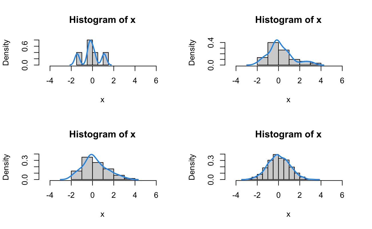
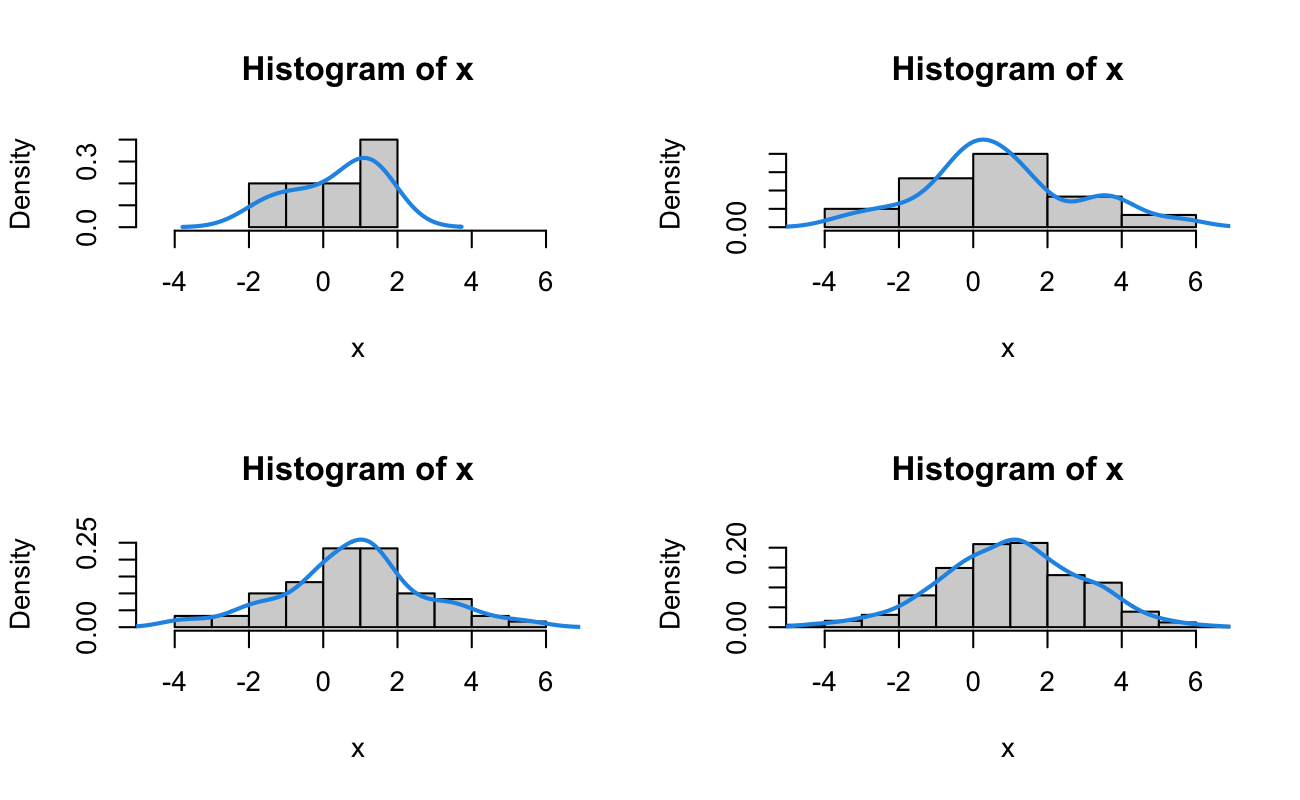
10.3 Example Random Samples
Code
set.seed(20150516)xStandard <-rnorm(n =1000, mean =0, sd =1)samplesStd_ls <-list(n5 = xStandard[1:5],n30 = xStandard[1:30],n60 = xStandard[1:60],n1000 = xStandard)xShift <-rnorm(n =1000, mean =1, sd =2)samplesShifted_ls <-list(n5 = xShift[1:5],n30 = xShift[1:30],n60 = xShift[1:60],n1000 = xShift)range_num <-range(c(xStandard, xShift))rm(xSymm, xSkew)Warning inrm(xSymm, xSkew): object 'xSymm' not foundWarning inrm(xSymm, xSkew): object 'xSkew' not found
After the absolutely Herculean task to derive this distribution, we have that it is a proper distribution by construction. It is nonnegative for all values of \(x \in \mathbb{R}\), and we constructed it so that \(\int_{\mathcal{S}(x)} dF(x|\mu, \sigma^2) = 1\).
10.5 Derive the Moment Generating Function
As we find the expectation of \(e^{tx}\), we will start with a \(w\)-substition as follows (I’m using \(w\) because \(u\) looks similar to \(\mu\) as I get more exhausted). Let \(w = \frac{x - \mu}{\sqrt{\sigma^2}}\), so \(dw = \frac{1}{\sqrt{\sigma^2}} dx \Rightarrow \sqrt{\sigma^2} dw = dx\), and \(x = w\sqrt{\sigma^2} + \mu\). The bounds of integration will not change. Now let’s begin our integration: \[
\begin{aligned}
M_x(t) &= \int_{\mathcal{S}(x)} e^{tx} dF(x|\mu, \sigma^2) \\
&= \int_{x = -\infty}^{\infty} e^{tx} \frac{1}{\sqrt{2\pi\sigma^2}} e^{-\frac{(x - \mu)^2}{2\sigma^2}} dx \\
&= \int_{w = -\infty}^{\infty} e^{t[w\sqrt{\sigma^2} + \mu]} \frac{1}{\sqrt{2\pi\sigma^2}} e^{-\frac{1}{2}[w]^2} [\sqrt{\sigma^2} dw] \\
&= \int_{-\infty}^{\infty} e^{tw\sqrt{\sigma^2}}e^{t\mu} \frac{1}{\sqrt{2\pi}} e^{-\frac{1}{2}w^2} dw \\
&= \frac{e^{t\mu}}{\sqrt{2\pi}} \int_{-\infty}^{\infty} e^{-\frac{1}{2}w^2 + tw\sqrt{\sigma^2}} dw.
\end{aligned}
\]
Notice that this yields a function with \(w^2\) and \(w\) in the exponent. We will use the technique of Completing the Square7 from preliminary algebra to factor this polynomial back into some function of \(w\) that is squared. Let’s pull out the exponent and work with it directly: \[
\begin{aligned}
\text{Exponent} &= -\frac{1}{2}w^2 + tw\sqrt{\sigma^2} \\
&= -\frac{1}{2}\left\{ w^2 - 2wt\sqrt{\sigma^2} \right\} \\
&= -\frac{1}{2}\left\{ w^2 - 2wt\sqrt{\sigma^2} + \left[t\sqrt{\sigma^2}\right]^2 - \left[t\sqrt{\sigma^2}\right]^2 \right\} \\
&= -\frac{1}{2}\left\{ \left( w^2 - 2wt\sqrt{\sigma^2} + \left[t\sqrt{\sigma^2}\right]^2 \right) - t^2\sigma^2 \right\} \\
&= -\frac{1}{2}\left\{ \left( w - t\sqrt{\sigma^2} \right)^2 - t^2\sigma^2 \right\} \\
&= -\frac{1}{2} \left( w - t\sqrt{\sigma^2} \right)^2 + \frac{1}{2} t^2\sigma^2 \\
\end{aligned}
\] Therefore, we continue our integration. We will quickly recognise the integral of the Normal Distribution with mean parameter \(t\sqrt{\sigma^2}\) and variance parameter \(1\). That is, \[
\begin{aligned}
M_x(t) &= \frac{e^{t\mu}}{\sqrt{2\pi}} \int_{-\infty}^{\infty} e^{-\frac{1}{2}w^2 + tw\sqrt{\sigma^2}} dw \\
&= \frac{e^{t\mu}}{\sqrt{2\pi}} \int_{-\infty}^{\infty} e^{-\frac{1}{2} \left( w - t\sqrt{\sigma^2} \right)^2 + \frac{1}{2} t^2\sigma^2} dw \\
&= e^{t\mu} \int_{-\infty}^{\infty} \frac{1}{\sqrt{2\pi}} e^{-\frac{1}{2} \left( w - t\sqrt{\sigma^2} \right)^2} e^{\frac{1}{2} t^2\sigma^2} dw \\
&= e^{t\mu + \frac{1}{2} t^2\sigma^2} \int_{-\infty}^{\infty} \frac{1}{\sqrt{2\pi}} e^{-\frac{1}{2} \left( w - t\sqrt{\sigma^2} \right)^2} dw \\
&= e^{t\mu + \frac{1}{2} t^2\sigma^2} \int_{-\infty}^{\infty} \mathcal{N}(w|t\sqrt{\sigma^2}, 1) dw \\
&= e^{t\mu + \frac{1}{2} t^2\sigma^2} [1] \\
&= \exp\left\{ t\mu + \frac{1}{2} t^2\sigma^2 \right\} \\
\end{aligned}
\]
10.6 Method of Moments Estimates from Observed Data
Let’s generate some random data. Let’s generate \(n = 7\) random IQ scores, which have mean 100 and standard deviation 15.8
Code
set.seed(20150516)IQmu <-100IQvar <-15^2rIQ_num <-rnorm(n =7, mean = IQmu, sd =sqrt(IQvar))
The 7 IQ scores are 116.4, 101.9, 95.1, 96.9, 78.3, 93.9, 98.1.
This bit is quite anti-climactic. The system to “solve” is \[
\mu = \bar{x};\ \sigma^2 = s^2.
\]Et voilà! We’re done.9
10.7 Maximum Likelihood Estimators
In comparison to the MGF section, this one will require a lot more work, and we will have to apply the Saddlepoint Test that we learned in the previous “Formal Foundations” chapter. So, for parameters \(\mu\) and \(\sigma^2\) (not \(\sigma\)), we find the log-likelihood in our traditional way: \[
\begin{aligned}
\mathcal{L}(\mu,\sigma^2|\textbf{x}) &= \prod_{i = 1}^n f(x_i|\mu, \sigma^2) \\
&= \prod_{i = 1}^n \frac{1}{\sqrt{2\pi\sigma^2}} e^{-\frac{(x_i - \mu)^2}{2\sigma^2}} \\
&= \prod_{i = 1}^n (2\pi)^{-1/2} (\sigma^2)^{-1/2} e^{-\frac{1}{2\sigma^2}(x_i - \mu)^2} \\
&= (2\pi)^{-n/2} (\sigma^2)^{-n/2} \exp\left\{-\frac{1}{2\sigma^2} \sum_{i = 1}^n (x_i - \mu)^2 \right\} \\
\Longrightarrow \ell(\mu,\sigma^2|\textbf{x}) &= \log\left( (2\pi)^{-n/2} (\sigma^2)^{-n/2} \exp\left\{-\frac{1}{2\sigma^2} \sum_{i = 1}^n (x_i - \mu)^2 \right\} \right) \\
&= -\frac{n}{2}\log(2\pi) - \frac{n}{2}\log(\sigma^2) - \frac{1}{2\sigma^2} \sum_{i = 1}^n (x_i - \mu)^2.
\end{aligned}
\]
Now, we have a function with two parameters, \(\mu\) and \(\sigma^2\). We will then have two first-order partial derivatives.
10.7.1 Candidate MLE for \(\mu\)
Let’s first take the derivative with respect to \(\mu\): \[
\begin{aligned}
\ell(\mu,\sigma^2|\textbf{x}) &= -\frac{n}{2}\log(2\pi) - \frac{n}{2}\log(\sigma^2) - \frac{1}{2\sigma^2} \sum_{i = 1}^n (x_i - \mu)^2 \\
\Longrightarrow \frac{\partial}{\partial\mu} \ell(\mu,\sigma^2|\textbf{x}) &= \frac{\partial}{\partial\mu} \left\{ -\frac{n}{2}\log(2\pi) - \frac{n}{2}\log(\sigma^2) - \frac{1}{2\sigma^2} \sum_{i = 1}^n (x_i - \mu)^2 \right\} \\
&= 0 - 0 - \frac{1}{2\sigma^2} \frac{\partial}{\partial\mu} \sum_{i = 1}^n (x_i^2 - 2x_i\mu + \mu^2) \\
&= -\frac{1}{2\sigma^2} \sum_{i = 1}^n \frac{\partial}{\partial\mu} (x_i^2 - 2x_i\mu + \mu^2) \\
&= -\frac{1}{2\sigma^2} \sum_{i = 1}^n (0 - 2x_i + 2\mu) \\
&= -\frac{1}{2\sigma^2} (-2n\bar{x} + 2n\mu) \\
&= \frac{n}{\sigma^2} (\bar{x} - \mu) \\
\Longrightarrow 0 &\overset{\text{set}}{=} \frac{n}{\sigma^2} (\bar{x} - \hat{\mu}_*) \\
\Longrightarrow \hat{\mu}_* &= \bar{x}.
\end{aligned}
\] Notice that I haven’t declared that this \(\hat{\mu}_*\) to be \(\hat{\mu}_{MLE}\). We still have to find our candidate value for \(\hat{\sigma}^2_*\) and then we have to check the second derivatives. So I’m leaving it as a “candidate” value for now.
10.7.2 Candidate MLE for \(\sigma^2\)
Similarly, we take the derivative with respect to \(\sigma^2\)\[
\begin{aligned}
\ell(\mu,\sigma^2|\textbf{x}) &= -\frac{n}{2}\log(2\pi) - \frac{n}{2}\log(\sigma^2) - \frac{1}{2\sigma^2} \sum_{i = 1}^n (x_i - \mu)^2 \\
\Longrightarrow \frac{\partial}{\partial\sigma^2} \ell(\mu,\sigma^2|\textbf{x}) &= \frac{\partial}{\partial\sigma^2} \left\{ -\frac{n}{2}\log(2\pi) - \frac{n}{2}\log(\sigma^2) - \frac{1}{2\sigma^2} \sum_{i = 1}^n (x_i - \mu)^2 \right\} \\
&= 0 -\frac{n}{2}\frac{1}{\sigma^2} - \frac{1}{2} \left[ \frac{\partial}{\partial\sigma^2} \frac{1}{\sigma^2} \right] \sum_{i = 1}^n (x_i - \mu)^2 \\
&= -\frac{n}{2\sigma^2} - \frac{1}{2} \left[ -\frac{1}{(\sigma^2)^2} \right] \sum_{i = 1}^n (x_i - \mu)^2 \\
&= \frac{1}{2(\sigma^2)^2} \sum_{i = 1}^n (x_i - \mu)^2 - \frac{n}{2\sigma^2} \\
\Longrightarrow 0 &\overset{\text{set}}{=} \frac{1}{2(\hat\sigma^2_*)^2} \sum_{i = 1}^n (x_i - \mu)^2 - \frac{n}{2\hat\sigma^2_*} \\
\Longrightarrow 2(\hat\sigma^2_*)^2 \times 0 &= 2(\hat\sigma^2_*)^2 \left[ \frac{1}{2(\hat\sigma^2_*)^2} \sum_{i = 1}^n (x_i - \mu)^2 - \frac{n}{2\hat\sigma^2_*} \right] \\
\Longrightarrow 0 &= \sum_{i = 1}^n (x_i - \mu)^2 - n\hat\sigma^2_* \\
\Longrightarrow n\hat\sigma^2_* &= \sum_{i = 1}^n (x_i - \mu)^2 \\
\Longrightarrow \hat\sigma^2_* &= \frac{1}{n}\sum_{i = 1}^n (x_i - \mu)^2.
\end{aligned}
\] So, we found a candidate MLE for \(\sigma^2\), but it depends on the unknown parameter \(\mu\). Also, we still don’t know that these two candidates actually maximise the likelihood function. We need the Hessian (matrix of second-order partial derivatives) for that.
10.7.3 The Hessian Matrix and its Determinant
As we alluded to previously (and spent an entire “Formal Foundations” section on), we will use the Saddlepoint Test to find out under what conditions these candidate values maximise the likelihood. Let’s find each of the second-order partial derivatives first. I’m going to start with the second derivative with respect to \(\sigma^2\) (and we notice that our candidate MLE for \(\sigma^2\) shows up at the end): \[
\begin{aligned}
\frac{\partial}{\partial\sigma^2} \ell(\mu,\sigma^2|\textbf{x}) &= \frac{1}{2(\sigma^2)^2} \sum_{i = 1}^n (x_i - \mu)^2 - \frac{n}{2\sigma^2} \\
\Longrightarrow \frac{\partial^2}{\partial(\sigma^2)^2} \ell(\mu,\sigma^2|\textbf{x}) &= \frac{\partial}{\partial\sigma^2} \left[ \frac{1}{2(\sigma^2)^2} \sum_{i = 1}^n (x_i - \mu)^2 - \frac{n}{2\sigma^2} \right] \\
&= -\frac{1}{(\sigma^2)^3} \frac{n}{n} \sum_{i = 1}^n (x_i - \mu)^2 + \frac{n}{2(\sigma^2)^2} \\
&= -\frac{n}{(\sigma^2)^2} \left[ \frac{1}{\sigma^2} \left( \frac{1}{n}\sum_{i = 1}^n (x_i - \mu)^2 \right) - \frac{1}{2} \right] \\
&= -\frac{n}{(\sigma^2)^2} \left[ \frac{\hat\sigma^2_*}{\sigma^2} - \frac{1}{2} \right].
\end{aligned}
\]
Now, we will take the crossing partial derivatives: \[
\begin{aligned}
\frac{\partial}{\partial\sigma^2} \ell(\mu,\sigma^2|\textbf{x}) &= \frac{1}{2(\sigma^2)^2} \sum_{i = 1}^n (x_i - \mu)^2 - \frac{n}{2\sigma^2} \\
\Longrightarrow \frac{\partial^2}{\partial\mu \partial\sigma^2} \ell(\mu,\sigma^2|\textbf{x}) &= \frac{\partial}{\partial\mu} \left[ \frac{1}{2(\sigma^2)^2} \sum_{i = 1}^n (x_i - \mu)^2 - \frac{n}{2\sigma^2} \right] \\
&= \frac{1}{2(\sigma^2)^2} \sum_{i = 1}^n \frac{\partial}{\partial\mu} (x_i - \mu)^2 - [0] \\
&= \frac{1}{2(\sigma^2)^2} \sum_{i = 1}^n \frac{\partial}{\partial\mu} (x_i^2 - 2x_i\mu + \mu^2) \\
&= \frac{1}{2(\sigma^2)^2} \sum_{i = 1}^n (-2x_i + 2\mu) \\
&= \frac{1}{(\sigma^2)^2} (-n\bar{x} + n\mu) \\
&= -\frac{n}{(\sigma^2)^2} (\bar{x} - \mu).
\end{aligned}
\] The other crossing partial should be equal to this one, but let’s confirm this: \[
\begin{aligned}
\frac{\partial}{\partial\mu} \ell(\mu,\sigma^2|\textbf{x}) &= \frac{n}{\sigma^2} (\bar{x} - \mu) \\
\Longrightarrow \frac{\partial^2}{\partial\sigma^2 \partial\mu} \ell(\mu,\sigma^2|\textbf{x}) &= \frac{\partial}{\partial\sigma^2} \frac{n}{\sigma^2} (\bar{x} - \mu) \\
&= -\frac{n}{(\sigma^2)^2} (\bar{x} - \mu).
\end{aligned}
\] The last partial derivative we need is with respect to \(\mu\) a second time: \[
\begin{aligned}
\frac{\partial}{\partial\mu} \ell(\mu,\sigma^2|\textbf{x}) &= \frac{n}{\sigma^2} (\bar{x} - \mu) \\
\Longrightarrow \frac{\partial^2}{\partial\mu^2} \ell(\mu,\sigma^2|\textbf{x}) &= \frac{\partial}{\partial\mu} \frac{n}{\sigma^2} (\bar{x} - \mu) \\
&= \frac{n}{\sigma^2}(-1) \\
&= -\frac{n}{(\sigma^2)^2} (\sigma^2).
\end{aligned}
\] This last step might seem counterproductive, but notice that all three of the other second-order partial derivatives had the same leading multiplier.
Now we can make the Hessian Matrix: \[
\textbf{H}[\ell(\mu,\sigma^2|\textbf{x})] = -\frac{n}{(\sigma^2)^2} \begin{bmatrix}
\sigma^2 & (\bar{x} - \mu) \\
(\bar{x} - \mu) & \left( \frac{\hat\sigma^2_*}{\sigma^2} - \frac{1}{2} \right)
\end{bmatrix}
\] Let’s inspect this matrix quickly. We don’t know what the determinant will be (yet), but we do know that the diagonal entries are both conditionally positive. Obviously \(\sigma^2 > 0\). Also, as long as \(\hat\sigma^2_* > \frac{1}{2}\sigma^2\), then the other diagonal component will be positive as well.10 This means that the negative sign outside has the same effect on both diagonal components. Thus, if the matrix \(\textbf{H}\) has a positive determinant, then we are dealing with a function that is concave down, and we will have found a local maximum. But again, this is a big “if”.
So what about this determinant? Before we take the determinant of this matrix, we should recall that for some square matrix \(\textbf{A}\in\mathbb{R}_p,\ \det(k\textbf{A}) = k^p\det(\textbf{A})\)11. Thus, the Hessian Determinant for all parameter values is: \[
\begin{aligned}
\det\left( \textbf{H}[\ell(\mu,\sigma^2|\textbf{x})] \right) &= \det \left( -\frac{n}{(\sigma^2)^2} \begin{bmatrix}
\sigma^2 & (\bar{x} - \mu) \\
(\bar{x} - \mu) & \left( \frac{\hat\sigma^2_*}{\sigma^2} - \frac{1}{2} \right)
\end{bmatrix} \right) \\
&= \left( -\frac{n}{(\sigma^2)^2} \right)^2 \left[ \sigma^2 \left( \frac{\hat\sigma^2_*}{\sigma^2} - \frac{1}{2} \right) - (\bar{x} - \mu)^2 \right] \\
&= \frac{n^2}{(\sigma^2)^4} \left[ \sigma^2 \left( \frac{\hat\sigma^2_*}{\sigma^2} - \frac{1}{2} \right) - (\bar{x} - \mu)^2 \right].
\end{aligned}
\] Now, let’s substitute in the candidate MLEs, \(\hat\mu_* = \bar{x}\) for \(\mu\) and \(\hat\sigma^2_* = \frac{1}{n}\sum_{i = 1}^n (x_i - \mu)^2\) for \(\sigma^2\). Delightfully, this simplifies nicely: \[
\begin{aligned}
\det\left( \textbf{H}[\ell(\mu = \hat\mu_*,\sigma^2 = \hat\sigma^2_*|\textbf{x})] \right) &= \frac{n^2}{[\hat\sigma^2_*]^4} \left[ [\hat\sigma^2_*] \left( \frac{\hat\sigma^2_*}{[\hat\sigma^2_*]} - \frac{1}{2} \right) - (\bar{x} - [\hat\mu_*])^2 \right] \\
&= \frac{n^2}{(\hat\sigma^2_*)^4} \left[ \hat\sigma^2_* \left( 1 - \frac{1}{2} \right) - (\bar{x} - \bar{x})^2 \right] \\
&= \frac{n^2}{(\hat\sigma^2_*)^4} \left[ \frac{1}{2}\hat\sigma^2_* \right] \\
&= \frac{n^2}{2(\hat\sigma^2_*)^3} \\
&> 0.
\end{aligned}
\]
10.7.4 MLEs Confirmed
Therefore, we have confirmed that the Hessian Matrix has “volume” at the critical points, and we saw above that the diagonal elements of the Hessian will both be negative (under the assumption that \(\hat\sigma^2_*\) isn’t a completely awful estimator for \(\sigma^2\)). Therefore, these critical points we found indeed maximize the likelihood function. Thus, \[
\hat\mu_{MLE} = \bar{x};\ \hat\sigma^2_{MLE} = \frac{1}{n}\sum_{i = 1}^n (x_i - \mu)^2.
\] For our real data, we don’t know \(\mu\), so these estimates are:
We generated data with a mean of 100 and a variance of \(15^2\) (which is 225). Our sample estimates are a mean of 97.2 and a variance of 109.1 (standard deviation of 10.4). Notice that I did not use the standard var() function. Why? This function calculates the sample standard deviation, \(s^2\), which is not the same as the MLE for \(\sigma^2\). In contrast, \(s^2\) for this data is
Code
var(rIQ_num)[1] 127
10.8 Exercises
10.8.1 The Log-Normal Distribution
If we let \(Y\sim\mathcal{N}(\mu, \sigma^2)\), and we let \(Y = \log(X)\), then \(X = e^Y\) has a Log-Normal distribution.
Use a transformation to find the PDF of this distribution. What is its support?
Show that \(\mathbb{E}[X] = e^{\mu + \frac{1}{2}\sigma^2}\).
Show that \(\text{Var}[X] = e^{2\mu + 2\sigma^2} - e^{2\mu + \sigma^2}\).
10.8.2 Simulating Properties of \(\sigma^2_{MLE}\)
While we were inspecting the Hessian Matrix above, we saw that \(\frac{\partial^2\ell}{\partial(\sigma^2)^2}\) includes the term \(\frac{\hat\sigma^2_*}{\sigma^2} - \frac{1}{2}\). Create a simulation study that increases the sample size and calculates this expression. How large of a sample (from a Normal distribution) would be required to be reasonably confident that this expression is positive?
This \(\textbf{0}\) will come from the same vector space as \(\boldsymbol\theta\). Also. this upside down triangle is called the “Del” or “nabla” symbol, and it denotes the vector of all possible first-order partial derivatives (because we don’t know how many dimensions the parameter space has). See https://en.wikipedia.org/wiki/Del↩︎
It’s technically a linear function, but that term has too many definitions. We need the “linear function” that means “non-affine”. See https://en.wikipedia.org/wiki/Linear_map↩︎
It may seem strange to you that I’m creating a “variance” object, and then immediately taking the square root of it. This is keeping in line with my derivation above that used \(\sigma^2\) as a symbol, rather than the quantity \(\sigma\) which has been squared. This will make our MLE work easier when we have to take the derivative with respect to the symbol \(\sigma^2\).↩︎
I have a severe complaint against Quarto for how I had to add the accent over the “a” here. The “default” fix to add a grave accent over a letter is to open the document in the visual editor, then insert the letter from a UTF library by the “Special Characters” option. From what I’ve found, there is currently no solution to add an accent over the letter by typing the traditional LaTeX command (\`{a}).↩︎
There is a homework exercise related to this question.↩︎