So far in our chapters, we have created quite a few likelihood functions. When we introduced likelihoods at the very beginning1, we were careful to state that likelihoods are not probability functions. However, we know two things:
likelihood functions are always non-negative (recall that the products of any number of non-negative numbers will still be non-negative), and
for well-behaved distributions, the area under the likelihood function will be finite (for a single finite data point from any well-behaved distribution, the parameter estimate for that data point will also be finite, and the product of finite values is finite).
Because the likelihood function is non-negative and the area under this curve is finite, we can turn it into a distribution by a process called finding the marginal likelihood2 and dividing the likelihood function by this marginal likelihood.
More formally, consider a probability function \(f(x|\boldsymbol{\theta})\) with some finite but unknown parameter vector \(\boldsymbol{\theta} \in\mathbb{R}_p\). Further, consider an independent and identical sample, \(\textbf{x}\), of size \(n\) from this distribution, represented as \(x_i \overset{iid}{\sim} f(x|\boldsymbol\theta),\ i = 1, 2, \ldots, n\). The resulting likelihood is \[
\mathcal{L}(\boldsymbol\theta|\textbf{x}) = \prod_{i = 1}^n f(x_i|\boldsymbol\theta).
\] In order to transform \(\mathcal{L}\) into a probability function, we must divide by the integral of \(\mathcal{L}\) over the support3 (all possible values) of \(\boldsymbol\theta\), where \(\mathcal{S}(\boldsymbol\theta)\) represents this support. For some distributions, especially those with a mixture of discrete and continuous parameters4, this support, \(\mathcal{S}(\boldsymbol\theta)\), may be quite complex.
Given this setup, the marginal likelihood is defined as \[
m(\boldsymbol\theta|\textbf{x}) = \int_{\mathcal{S}(\boldsymbol\theta)} \mathcal{L}(\boldsymbol\theta|\textbf{x}) \pi(\boldsymbol\theta) d\boldsymbol\theta.
\] This \(\pi(\boldsymbol\theta)\) may come as a surprise, as we haven’t defined what it is. In Bayesian Statistics5, this \(\pi(\boldsymbol\theta)\) is known as a prior distribution6. In the context of Bayesian inference, this prior distribution represents all the expert knowledge about the unknown parameter vector \(\boldsymbol\theta\) that was known before the sample \(\textbf{x}\) was collected. However, for this class, we will make the statement that we don’t know much, if anything, about \(\boldsymbol\theta\), so we set \(\pi(\boldsymbol\theta) = 1\). Then, for our examples, \[
m(\boldsymbol\theta|\textbf{x}) = \int_{\mathcal{S}(\boldsymbol\theta)} \mathcal{L}(\boldsymbol\theta|\textbf{x}) d\boldsymbol\theta.
\]
Finally, in order to transform the likelihood function of \(\boldsymbol\theta\) into a probability function of \(\boldsymbol\theta\), we will divide the likelihood by its integral. So, the probability function of \(\boldsymbol\theta\) given the observed data \(\textbf{x}\) is \[
f(\boldsymbol\theta|\textbf{x}) = \frac{\mathcal{L}(\boldsymbol\theta|\textbf{x})}{m(\boldsymbol\theta|\textbf{x})} = \frac{\mathcal{L}(\boldsymbol\theta|\textbf{x})}{\int_{\mathcal{S}(\boldsymbol\theta)} \mathcal{L}(\boldsymbol\theta|\textbf{x}) d\boldsymbol\theta}.
\] We comment that distributions derived this way are true statistical distributions because they will always be non-negative, and an integral divided by itself equals 1 (so the total probability will be 1 by definition). In practice, this integral may be impossible to solve, so often numerical routines are used to estimate \(f\) directly. Such topics are beyond the scope of this course.
8.1.2 Fubini’s Theorem
One small piece of theory we will need below is to swap the order of integration and summation (which we have done quite loosely up to this point). Basically, if we have two properties: 1) that \(f \ge 0\), and \(F < \infty\), then \[
\int \sum_n f_n(x) dx = \sum_n \int f_n(x) dx.
\] This is an extension of Fubini’s Theorem7 which allows us to swap the order of summation and integration, as long as the function \(f\) is non-negative and the integral converges. Note that if \(f\) is a probability function of a statistical distribution, then we have both properties automatically.
8.2 Deriving the Distribution
We will begin this process by considering an independent and identical sample \(\textbf{x}\), with size \(n\), from an Binomial Distribution (with \(p\) unknown); that is \(x_i \overset{iid}{\sim} \text{Binom}(N, p),\ i = 1, 2, \ldots, n\). Further, we will take a play from the Negative Binomial distribution, and let \(k_i\) and \(r_i\) denote the number of successes and failures in Binomial sample \(i\), respectively. Thus, \[
\begin{align}
\mathcal{L}(p|\textbf{x}) &= \prod_{i = 1}^n {N \choose x_i} p^{x_i} (1 - p)^{N - x_i} \\
\Longrightarrow \mathcal{L}(p|\textbf{r},\textbf{k}) &= \prod_{i = 1}^n {r_i + k_i \choose k_i} p^{k_i} (1 - p)^{r_i} \\
&= \left[ \prod_{i = 1}^n {r_i + k_i \choose k_i} \right] \times \left[ \prod_{i = 1}^n p^{k_i} \right] \times \left[ \prod_{i = 1}^n (1 - p)^{r_i} \right] \\
&= \left[ \prod_{i = 1}^n {r_i + k_i \choose k_i} \right] p^{S_k} (1 - p)^{S_r},
\end{align}
\] where \[
S_k = \sum_{i = 1}^n k_i,\ \text{and}\ S_r = \sum_{i = 1}^n r_i.
\]
As we discussed in our Formal Foundations section, we can marginalize this likelihood to create a probability function \(f\), of the parameter \(p\), given the sufficient statistics8 of the observed data \(S_k\) and \(S_r\). That is, \[
\begin{align}
f(p|S_r, S_k) &= \frac{\mathcal{L}(p|\textbf{r},\textbf{k})}{m(p|\textbf{r},\textbf{k})} \\
&= \frac{\mathcal{L}(p|\textbf{r},\textbf{k})}{\int_{\mathcal{S}(p)} \mathcal{L}(p|\textbf{r},\textbf{k}) dp } \\
&= \frac{ \left[ \prod_{i = 1}^n {r_i + k_i \choose k_i} \right] p^{S_k} (1 - p)^{S_r} }{\int_0^1 \left[ \prod_{i = 1}^n {r_i + k_i \choose k_i} \right] p^{S_k} (1 - p)^{S_r} dp } \\
&= \frac{ \left[ \prod_{i = 1}^n {r_i + k_i \choose k_i} \right] p^{S_k} (1 - p)^{S_r} }{ \left[ \prod_{i = 1}^n {r_i + k_i \choose k_i} \right] \int_0^1 p^{S_k} (1 - p)^{S_r} dp } \\
&= \frac{ p^{S_k} (1 - p)^{S_r} }{ \int_0^1 p^{S_k} (1 - p)^{S_r} dp } \\
&= \frac{ p^{(S_k + 1) - 1} (1 - p)^{(S_r + 1) - 1} }{ \int_0^1 p^{(S_k + 1) - 1} (1 - p)^{(S_r + 1) - 1} dp } \\
&= \frac{ p^{\alpha - 1} (1 - p)^{\beta - 1} }{ \int_0^1 p^{\alpha - 1} (1 - p)^{\beta - 1} dp },
\end{align}
\] where \(\alpha = S_k + 1\) (1 plus the total number of successes in the \(n\) Binomial trials) and \(\beta = S_r + 1\) (1 plus the total number of failures in the \(n\) Binomial trials).
This integral in the denominator should look familiar: it is the definition of the Complete Beta Function, which we covered in the “Formal Foundations” chapter on the Gamma and Beta functions. Thus, \[
\begin{align}
f(p|S_r, S_k) &= \frac{ p^{\alpha - 1} (1 - p)^{\beta - 1} }{ \int_0^1 p^{\alpha - 1} (1 - p)^{\beta - 1} dp } \\
&= \left[ \int_0^1 p^{\alpha - 1} (1 - p)^{\beta - 1} dp \right]^{-1} p^{\alpha - 1} (1 - p)^{\beta - 1} \\
&= \left[ \frac{\Gamma(\alpha)\Gamma(\beta)}{\Gamma(\alpha + \beta)} \right]^{-1} p^{\alpha - 1} (1 - p)^{\beta - 1} \\
&= \frac{\Gamma(\alpha + \beta)}{\Gamma(\alpha)\Gamma(\beta)} p^{\alpha - 1} (1 - p)^{\beta - 1},
\end{align}
\] which is the standard form of the Beta Distribution with \(p\in(0,1)\).
What are the allowed values for \(\alpha\) and \(\beta\)? Because we derived the Beta Distribution as the probability function of the Binomial Distribution’s parameter \(p\), we had an added restriction that \(S_k\) and \(S_r\) were non-negative integers (that is, \(S_k,\ S_r \in 0\cup\mathbb{N} = 0, 1, 2, 3, \ldots\)). This would impose the restriction that \(\alpha = S_k + 1\) and \(\beta = S_r + 1\) must be elements of \(\mathbb{N} = 1, 2, 3, \ldots\) (not including 0). However, notice that the form of \(f\) above uses Gamma functions, so it does not require that \(\alpha\) and \(\beta\) be restricted to the integers. What would it mean to have fractional/decimal counts of successes or failures? Well, some games allow for ties, which could be counted as half a success and half a failure. Other experiments could involve Likert-scale9 responses, where “strongly disagree” maps to 0, “strongly agree” maps to 1, but the values in between map to various fractions between 0 and 1.10 Thus, we state that \(\alpha\) and \(\beta\) simply need to be non-negative real numbers (\(\alpha,\beta\in\mathbb{R}^+\)).
Given all our work to derive this distribution, we can show that it is a distribution directly. First, note that because \(p\in(0,1)\) and \(\alpha,\beta > 0\), we have that \(f(p|\alpha,\beta) > 0\). Then, starting with the Riemann-Stieltjes integral and applying the definition of the Complete Beta Function11 we have \[
\begin{align}
\int_{\mathcal{S}(p)} dF(p|\alpha,\beta) &= \int_0^1 \frac{\Gamma(\alpha + \beta)}{\Gamma(\alpha)\Gamma(\beta)} p^{\alpha - 1} (1 - p)^{\beta - 1} dp \\
&= \frac{\Gamma(\alpha + \beta)}{\Gamma(\alpha)\Gamma(\beta)} \int_0^1 p^{\alpha - 1} (1 - p)^{\beta - 1} dp \\
&= \frac{\Gamma(\alpha + \beta)}{\Gamma(\alpha)\Gamma(\beta)} \left[ \frac{\Gamma(\alpha)\Gamma(\beta)}{\Gamma(\alpha + \beta)} \right] \\
&= 1.
\end{align}
\] Therefore, the Beta Distribution is a proper distribution.
8.5 Derive the Moment Generating Function
When I was in grad school, some of my professors ignored deriving the Moment Generating Function of the Beta Distribution. When you look at its form in the back of a statistical theory textbook, you can probably see why (it’s unpleasant). However, we are going to derive it anyway. Many derivations you might find online involve using the Kummer’s Function of the First Kind12, which requires even more theoretical foundations to cover than I would ever want to write. Instead, we will opt for a longer derivation, but one that uses Formal Foundations that we have already covered, namely the Riemann-Stieljes Integral (that you should be comfortable with by now), the MacLaurin Series13 of \(e^x\), swapping the order of integration and summation via Fubini’s Theorem,14 the definition of the Complete Beta Function,15 and the Continued Recurrence Property of the Gamma Function.16
Let’s begin: \[
\begin{aligned}
M_p(t) &= \int_{\mathcal{S}(p)} e^{tp}dF(p|\alpha,\beta) \\
&= \int_0^1 e^{tp} \frac{\Gamma(\alpha + \beta)}{\Gamma(\alpha)\Gamma(\beta)} p^{\alpha - 1} (1 - p)^{\beta - 1} dp \\
&\qquad\text{\emph{MacLaurin Series of }} e^{tp} \text{\emph{...}} \\
&= \frac{\Gamma(\alpha + \beta)}{\Gamma(\alpha)\Gamma(\beta)} \int_0^1 \left[ \sum_{k = 0}^{\infty} \frac{(tp)^k}{k!} \right] p^{\alpha - 1} (1 - p)^{\beta - 1} dp \\
&= \frac{\Gamma(\alpha + \beta)}{\Gamma(\alpha)\Gamma(\beta)} \int_0^1 \sum_{k = 0}^{\infty} \frac{t^k}{k!} p^k p^{\alpha - 1} (1 - p)^{\beta - 1} dp \\
&\qquad\text{\emph{Fubini's Theorem...}} \\
&= \frac{\Gamma(\alpha + \beta)}{\Gamma(\alpha)\Gamma(\beta)} \sum_{k = 0}^{\infty} \int_0^1 \frac{t^k}{k!} p^k p^{\alpha - 1} (1 - p)^{\beta - 1} dp \\
&= \frac{\Gamma(\alpha + \beta)}{\Gamma(\alpha)\Gamma(\beta)} \sum_{k = 0}^{\infty} \frac{t^k}{k!} \int_0^1 p^{\alpha + k - 1} (1 - p)^{\beta - 1} dp \\
&\qquad\text{\emph{Defn. of Beta Function...}} \\
&= \frac{\Gamma(\alpha + \beta)}{\Gamma(\alpha)\Gamma(\beta)} \sum_{k = 0}^{\infty} \frac{t^k}{k!} \left[ \frac{\Gamma(\alpha + k)\Gamma(\beta)}{\Gamma(\alpha + \beta + k)} \right] \\
&= \sum_{k = 0}^{\infty} \frac{t^k}{k!} \left[ \frac{\Gamma(\alpha + \beta)}{\Gamma(\alpha + \beta + k)} \frac{\Gamma(\alpha + k)}{\Gamma(\alpha)} \right] \\
&\qquad\text{\emph{``Peel off'' the first summand...}} \\
&= \frac{t^0}{0!} \left[ \frac{\Gamma(\alpha + \beta)}{\Gamma(\alpha + \beta + 0)} \frac{\Gamma(\alpha + 0)}{\Gamma(\alpha)} \right] + \sum_{k = 1}^{\infty} \frac{t^k}{k!} \left[ \frac{\Gamma(\alpha + \beta)}{\Gamma(\alpha + \beta + k)} \frac{\Gamma(\alpha + k)}{\Gamma(\alpha)} \right] \\
&\qquad\text{\emph{Gamma Function Recurrence Property...}} \\
&= 1 + \sum_{k = 1}^{\infty} \frac{t^k}{k!} \left[ \frac{\Gamma(\alpha + \beta)}{ \prod_{j = 0}^{k - 1} (\alpha + \beta + j) \Gamma(\alpha + \beta) } \frac{ \prod_{j = 0}^{k - 1} (\alpha + j) \Gamma(\alpha) }{\Gamma(\alpha)} \right] \\
&= 1 + \sum_{k = 1}^{\infty} \frac{t^k}{k!} \left[ \frac{1}{ \prod_{j = 0}^{k - 1} (\alpha + \beta + j) } \frac{ \prod_{j = 0}^{k - 1} (\alpha + j) }{1} \right] \\
&= 1 + \sum_{k = 1}^{\infty} \frac{t^k}{k!} \left[ \prod_{j = 0}^{k - 1} \frac{\alpha + j}{\alpha + \beta + j} \right],
\end{aligned}
\] which is the standard form of the Beta Distribution’s MGF. We “peeled off” the first summand (incrementing from \(k = 0\) to \(k = 1\)) to make taking the first derivative easier. When we are ready to take the second derivative, we will “peel off” the second summand (incrementing from \(k = 1\) to \(k = 2\)) then.
8.6 Method of Moments Estimates from Observed Data
8.6.1 Effect of \(\alpha\) and \(\beta\) on Sampled Probabilities
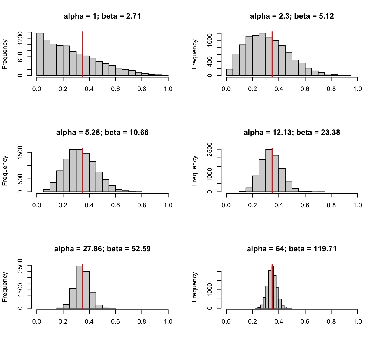
Following our Binomial example with probability of success \(p_0 = 0.35\), let’s create a probability distribution from which this \(p_0\) is the most likely value. For the Beta Distribution, the formula for the mode17 is known, so we set it equal to 0.35, and we will have a frontier18 where one unknown variable can be written as a function of another: \[
\begin{aligned}
0.35 &= \frac{\alpha - 1}{\alpha + \beta - 2} \\
\Longrightarrow 0.35\alpha + 0.35\beta - 0.7 &= \alpha - 1 \\
\Longrightarrow 0.35\beta &= 0.65\alpha - 0.3 \\
\Longrightarrow \beta(\alpha) = \frac{13}{7}\alpha + \frac{6}{7}.
\end{aligned}
\] Notice that if we pick a value for one parameter of the Beta Distribution, while holding the mode constant, then the other value is determined.
Let’s pick a range of values for \(\alpha\), calculate the corresponding values of \(\beta\), and then look at the distribution of values as \(\alpha\) and \(\beta\) increase.
Notice that for small values of \(\alpha\), the mode of the distribution is not the desired 0.35. However, as \(\alpha\) grows larger, the mode both gets closer to 0.35 and the distribution gets tighter around the desired value of 0.35.
The intuition for this goes back to the motivating derivation of the Beta Distribution. The parameters \(\alpha\) and \(\beta\) represent the total number of successes and failures, respectfully, in repeated independent Binomial experiments. The more total successes and failures we’ve observed, the more information we have about the true value of \(p\). Therefore, the distribution must shrink and become more narrow around the intended value of \(p_0 = 0.35\). In practice, larger parameters of the Beta Distribution represent more prior information known about the probability of success, \(p\).
8.6.2 A “Random Sample” of Probabilities
Let’s generate some random data. Before we do this, we should think critically about this exercise. When, if ever, is it truly possible to “observe” a probability? We can observe successes and failures, but in the health science context, I can’t think of any case where we could actually take a random sample of probabilities themselves. However, this somewhat nonsensical step is necessary to move forward with our examples for the Method of Moments estimators and also to describe the forms of the solutions to the MLE exercises. So, we will press onward.
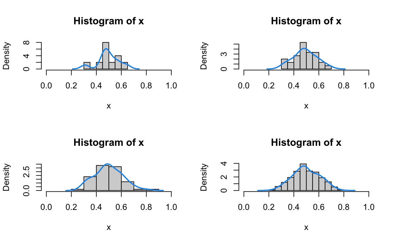
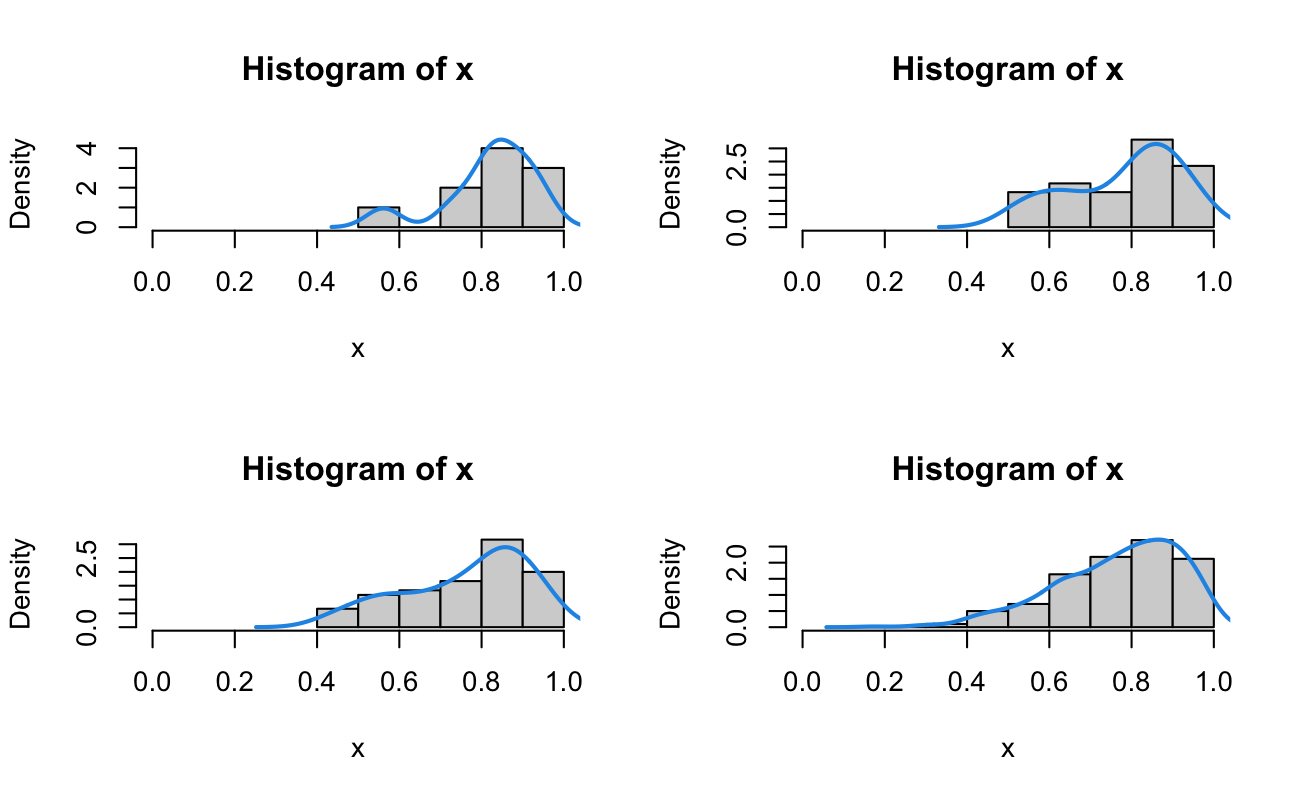
We will assume that we already know that in prior independent Binomial experiments, we observed a total of 64 successes and 120 failures. Let’s assume that we somehow “observed” \(n = 12\) probabilities from a Beta distribution with \(\alpha = 64 + 1\) and \(\beta = 120 + 1\). This would yield a theoretical mode value of \((65 - 1)/(65 + 121 - 2) \approx 0.348\). We can sample these values as shown below:
After these derivations, we have the following system of equations: \[
\bar{p} = \frac{\alpha}{\alpha + \beta};\ s^2 = \frac{\alpha\beta}{(\alpha + \beta)^2(\alpha + \beta + 1)}.
\] Let’s solve the first equation for \(\beta\), since it only appears once: \[
\begin{aligned}
\bar{p} &= \frac{\alpha}{\alpha + \beta} \\
\Longrightarrow \alpha\bar{p} + \beta\bar{p} &= \alpha \\
\Longrightarrow \beta\bar{p} &= \alpha - \alpha\bar{p} \\
\Longrightarrow \beta &= \frac{\alpha}{\bar{p}} - \alpha.
\end{aligned}
\]
We will now substitute this value for \(\beta\), which depends on the known value of \(\bar{p}\) and the unknown value of \(\alpha\), into the second equation: \[
\begin{aligned}
s^2 &= \frac{\alpha\beta}{(\alpha + \beta)^2(\alpha + \beta + 1)} \\
&= \frac{\alpha\left[ \frac{\alpha}{\bar{p}} - \alpha \right]}{\left(\alpha + \left[ \frac{\alpha}{\bar{p}} - \alpha \right]\right)^2 \left(\alpha + \left[ \frac{\alpha}{\bar{p}} - \alpha \right] + 1\right)} \\
&= \frac{ \alpha^2\left[ \frac{1}{\bar{p}} - 1 \right] }{\left( \frac{\alpha}{\bar{p}} \right)^2 \left( \frac{\alpha}{\bar{p}} + 1 \right)} \\
&= \frac{ \alpha^2\left[ \frac{1}{\bar{p}} - 1 \right] }{ \alpha^2 \left( \frac{\alpha}{\bar{p}^3} + \frac{1}{\bar{p}^2} \right)} \times \frac{\bar{p}^3}{\bar{p}^3} \\
&= \frac{ \left[ 1 - \bar{p} \right] \bar{p}^2 }{ \frac{\alpha\bar{p}^3}{\bar{p}^3} + \frac{\bar{p}^3}{\bar{p}^2} } \\
&= \frac{ (1 - \bar{p})\bar{p}^2 }{\alpha + \bar{p}} \\
\Longrightarrow s^2(\alpha + \bar{p}) &= (1 - \bar{p})\bar{p}^2 \\
\Longrightarrow s^2\alpha &= (1 - \bar{p})\bar{p}^2 - s^2\bar{p} \\
\Longrightarrow \hat{\alpha} &= (1 - \bar{p})\frac{\bar{p}^2}{s^2} - \bar{p}.
\end{aligned}
\]
Finally, we can substitute this estimate for \(\alpha\), which is entirely in terms of the known quantities \(\bar{p}\) and \(s^2\), back into the first equation that we solved for \(\beta\). Thus, \[
\begin{aligned}
\beta &= \frac{\alpha}{\bar{p}} - \alpha \\
&= \left[ \alpha \right]\left[ \frac{1}{\bar{p}} - 1 \right] \\
\Longrightarrow \hat{\beta} &= \left[ (1 - \bar{p})\frac{\bar{p}^2}{s^2} - \bar{p} \right] \left[ \frac{1}{\bar{p}} - 1 \right].
\end{aligned}
\]
Now that we have these two equations in terms of the known quantities, we can find the Method of Moments estimates for \(\alpha\) and \(\beta\) given the \(n = 12\) “observed” data points:
So, while the true parameter values used to generate this sample of \(n = 12\) probabilities were \(\alpha\) = 65 and \(\beta\) = 121, our Method of Moments estimates are \(\hat{\alpha}\) = 86.7 and \(\hat{\beta}\) = 166.7.
8.7 Maximum Likelihood Estimators
We have similar qualms here as in the Method of Moments section, in that it’s a strange thing to think about “observing” probabilities. However, we can still work through some of the MLE steps for the Beta Distribution. Let \(\textbf{p} = p_1, p_2, \ldots, p_n\) be an independent and identical sample from a Beta Distribution with unknown parameters \(\alpha\) and \(\beta\). We start with the Likelihood function: \[
\begin{aligned}
\mathcal{L}(\alpha, \beta|\textbf{p}) &= \prod_{i = n}^n \frac{\Gamma(\alpha + \beta)}{\Gamma(\alpha)\Gamma(\beta)} p_i^{\alpha - 1} (1 - p_i)^{\beta - 1} \\
\Longrightarrow \ell(\alpha, \beta|\textbf{p}) &= \sum_{i = 1}^n \log \left[ \frac{\Gamma(\alpha + \beta)}{\Gamma(\alpha)\Gamma(\beta)} p_i^{\alpha - 1} (1 - p_i)^{\beta - 1} \right] \\
&= \sum_{i = 1}^n \left\{ \log \left[ \frac{\Gamma(\alpha + \beta)}{\Gamma(\alpha)\Gamma(\beta)} \right] + \log \left[ p_i^{\alpha - 1} \right] + \log \left[ (1 - p_i)^{\beta - 1} \right] \right\} \\
&= n\log \left[ \frac{\Gamma(\alpha + \beta)}{\Gamma(\alpha)\Gamma(\beta)} \right] + (\alpha - 1) \sum_{i = 1}^n \log(p_i) + (\beta - 1)\sum_{i = 1}^n \log(1 - p_i).
\end{aligned}
\]
We immediately see two problems:
We are taking the partial derivatives with respect to \(\alpha\) and \(\beta\), which are inside of Gamma functions, so we will not have a closed-form solution regardless.
The \(\Gamma(\alpha + \beta)\) term is a single Gamma function with both \(\alpha\) and \(\beta\) inside, so any partial derivatives with respect to one variable will still contain the other variable. These parameters cannot be estimated independently.
The partial derivative with respect to \(\alpha\) is found by: \[
\begin{aligned}
\ell(\alpha, \beta|\textbf{p}) &= n\log \left[ \frac{\Gamma(\alpha + \beta)}{\Gamma(\alpha)\Gamma(\beta)} \right] + (\alpha - 1) \sum_{i = 1}^n \log(p_i) + (\beta - 1)\sum_{i = 1}^n \log(1 - p_i) \\
&= n\log \left[ \frac{\Gamma(\alpha + \beta)}{\Gamma(\alpha)} \right] - n\log \left[ \Gamma(\beta) \right] + (\alpha - 1) \sum_{i = 1}^n \log(p_i) + (\beta - 1)\sum_{i = 1}^n \log(1 - p_i) \\
\Longrightarrow \frac{\partial}{\partial \alpha} \ell(\alpha, \beta|\textbf{p}) &= n \frac{\partial}{\partial \alpha} \log \left[ \frac{\Gamma(\alpha + \beta)}{\Gamma(\alpha)} \right] - [0] + \sum_{i = 1}^n \log(p_i) + [0] \\
&= n \frac{\partial}{\partial \alpha} \log \left[ \frac{\Gamma(\alpha + \beta)}{\Gamma(\alpha)} \right] + n\overline{\log(p)} \\
0 &\overset{\text{set}}{=} n \frac{\partial}{\partial \alpha} \log \left[ \frac{\Gamma(\alpha + \beta)}{\Gamma(\alpha)} \right] + n\overline{\log(p)} \\
\Longrightarrow -\overline{\log(p)} &= \frac{\partial}{\partial \alpha} \log \left[ \frac{\Gamma(\alpha + \beta)}{\Gamma(\alpha)} \right].
\end{aligned}
\] We can’t get much further than this analytically. If either \(\alpha\) or \(beta\) are known to be an integer (for instance, if we know that these parameters truly represent integer counts of successes and failures in prior studies), then we can employ the Continued Recurrence Property of the Gamma Function as follows (but it doesn’t make the problem much easier): \[
\begin{aligned}
-\overline{\log(p)} &= \frac{\partial}{\partial \alpha} \log \left[ \frac{\Gamma(\alpha + \beta)}{\Gamma(\alpha)} \right] \\
&= \frac{\partial}{\partial \alpha} \log \left[ \frac{\Gamma(\alpha) \prod_{j = 0}^{\beta - 1} (\alpha + j)}{\Gamma(\alpha)} \right] \\
&= \frac{\partial}{\partial \alpha} \log \left[ \prod_{j = 0}^{\beta - 1} (\alpha + j) \right] \\
&= \frac{\partial}{\partial \alpha} \sum_{j = 0}^{\beta - 1} \log (\alpha + j) \\
&= \sum_{j = 0}^{\beta - 1} \frac{\partial}{\partial \alpha} \log (\alpha + j) \\
&= \sum_{j = 0}^{\beta - 1} \frac{1}{\alpha + j} \\
&= \frac{1}{\alpha} + \frac{1}{\alpha + 1} + \ldots + \frac{1}{\alpha + \beta - 1}.
\end{aligned}
\] Now, this may look easier to work with (and it is easier computationally, because this is a smooth, positive, decreasing function for \(\alpha > 0\)), but notice that the unknown parameter \(\beta\) is now in the support of the computation for \(\alpha\). So, we are still in a situation where we need to estimate one parameter first in order to approximate a value for the second. If we have a guess for \(\beta\) then this becomes a manageable coding problem to estimate \(\alpha\). Also, note that because \(p\in(0,1)\), \(-\overline{\log(p)} \in (0,\infty)\), so there will be a solution to the problem.
We now have a system of two equations and two unknowns (assuming that we can limit \(\alpha\) and \(\beta\) to the integers—if we cannot, then we have to use the Digamma functions19). That system is: \[
-\overline{\log(p)} = \sum_{j = 0}^{\beta - 1} \frac{1}{\alpha + j};\quad -\overline{\log(1 - p)} = \sum_{j = 0}^{\alpha - 1} \frac{1}{\beta + j}.
\] Theoretically, we could solve this numerically. Often, we would use the Method of Moments estimates as the initial values for \(\alpha\) and \(\beta\).
8.8 Exercises
8.8.1 The Uniform Distribution
The Continuous Uniform Distribution over \((0,1)\) is a special case of the Beta Distribution with \(\alpha = 1\) and \(\beta = 1\).
Show that the Uniform Distribution is a proper distribution.
Show that the MGF is \(M_p(t) = \frac{1}{t}(e^t - 1)\).
Find \(\mathbb{E}[p]\) and \(\text{Var}[p]\).
8.8.2 Computational Solution to the MLEs
Try to write some code that will estimate \(\alpha\) and \(\beta\) from a vector of known “observed” probabilities, \(\textbf{p}\).
For example, the Negative Binomial distribution has parameter vector \(\langle n,p \rangle\) when \(n\) is unknown, where \(p\in (0,1)\) and \(n\in\mathbb{N}\).↩︎