1  The Bernoulli Distribution

1.1 Background

The Bernoulli distribution is one of the simplest yet most fundamental probability distributions in statistics. Named after Jacob Bernoulli, who pioneered probability theory in the 17th century, it describes random experiments that result in only two possible outcomes: success (usually coded as 1) and failure (coded as 0). The probability of success is denoted by p, and the probability of failure is \(1 - p\), with \(0 < p < 1\).

Despite its simplicity, the Bernoulli distribution forms the cornerstone of many important statistical methods. It is the basis for the binomial distribution (sum of Bernoulli trials), the geometric distribution (number of trials until the first success), and the negative binomial distribution (number of trials until a fixed number of successes). In biostatistics, it is particularly relevant because many biomedical and public health variables are binary in nature, such as presence/absence of disease, treatment success/failure, or survival/death (Johnson, Kemp, and Kotz (2005)).

1.1.1 Applications in Biostatistics

The Bernoulli distribution is widely used in biostatistical research, particularly when analyzing binary outcomes:

• Epidemiology: Disease status (infected vs. not infected), exposure status (exposed vs. not exposed), or vaccination uptake (yes/no) (Agegnehu and Alem (2021)).
• Clinical Trials: Treatment response (success vs. failure), adverse event occurrence, or survival within a fixed period (Branson and Bind (2019)).
• Public Health Surveys: Yes/no responses in questionnaires (e.g., smoker vs. non-smoker, exercised vs. not exercised) (Abbasi, Shad, and Ahmed (2022)).
• Logistic Regression: Logistic regression assumes the response variable follows a Bernoulli distribution conditional on predictors, making it the theoretical backbone of modeling binary health outcomes (Hosmer, Lemeshow, and Sturdivant (2013)).
• Survival Analysis: The censoring indicator in survival studies (event occurred = 1, censored = 0) follows a Bernoulli distribution, forming the basis for event-time modeling (Xue and Brookmeyer (1997)).

1.2 Deriving the Distribution

In the mid-1600s, mathematicians like Pascal and Fermat were obsessed with games of chance.¹ The simplest such game is flipping a single coin. Let \(P[A]\) denote the probability of event \(A\) occurring. Because flipping a coin has only two outcomes (heads or tails; we ignore the microscopic possibility of a coin landing on its edge for practical gambling scenarios), we can define \(p \equiv P[\text{head}]\), which necessarily implies that \(1 - p = P[\text{tails}]\). For ease of notation, we let \(k\in\{0,1\} = 1\) when the coin hands on leads and \(k = 0\) for tails. Thus, we define a Bernoulli Trial as one random value drawn from the following distribution: \[ f_{\text{Bern}}(k|p) = p^k(1-p)^{1-k},\ k\in\{0,1\},\ p \in (0,1) \subset \mathbb{R}. \]

Notice a few things:

• The Bernoulli Probability Mass Function is denoted \(f_{\text{Bern}}\); \(f\) is a function, and its argument \(k\) is discrete. The domain of \(f\) is 0 or 1 (\(k\) can only have the values in the set \(\mathcal{S} = \{0,1\}\)).
• For any \(k \in \mathcal{S}\), \(f(k|p) \ge 0\); this is the range of \(f\). This means that \(f\) maps from the set \(\mathcal{S}\) to the set of all non-negative real numbers, which is symbolically denoted as \(f:\mathcal{S} \to \mathbb{R}_{\ge}\).
• The probability of a “head” (success) is the only parameter of \(f\), and it is fixed at some value \(p\), which must be a real number between 0 and 1.

1.2.1 An Example Sample from the Bernoulli Distribution

Now let’s use R to take \(n = 100\) random samples from a Bernoulli Distribution with \(p = 0.35\), but we will only inspect the first five (for now):

set.seed(20150516)
myBernSample <- rbinom(n = 100, size = 1, prob = 0.35)
myBernSample[1:5]
[1] 1 0 0 1 0

We now pretend that we only know the results for the first five coin flips. We have flipped one coin five times, with the results \(\{\)Heads, Tails, Heads, Tails, Tails\(\}\).

1.3 Example Random Samples

We now take some random samples from this distribution when \(p = 0.5\).

set.seed(20150516)

x <- rbinom(n = 100, size = 1, prob = 0.5)
samples_ls <- list(
  n5   = x[1:5],
  n15  = x[1:15],
  n30  = x[1:30],
  n100 = x
)

rm(x)

par(mfrow = c(2, 2))

hist(samples_ls$n5)
hist(samples_ls$n15)
hist(samples_ls$n30)
hist(samples_ls$n100)

par(mfrow = c(1, 1))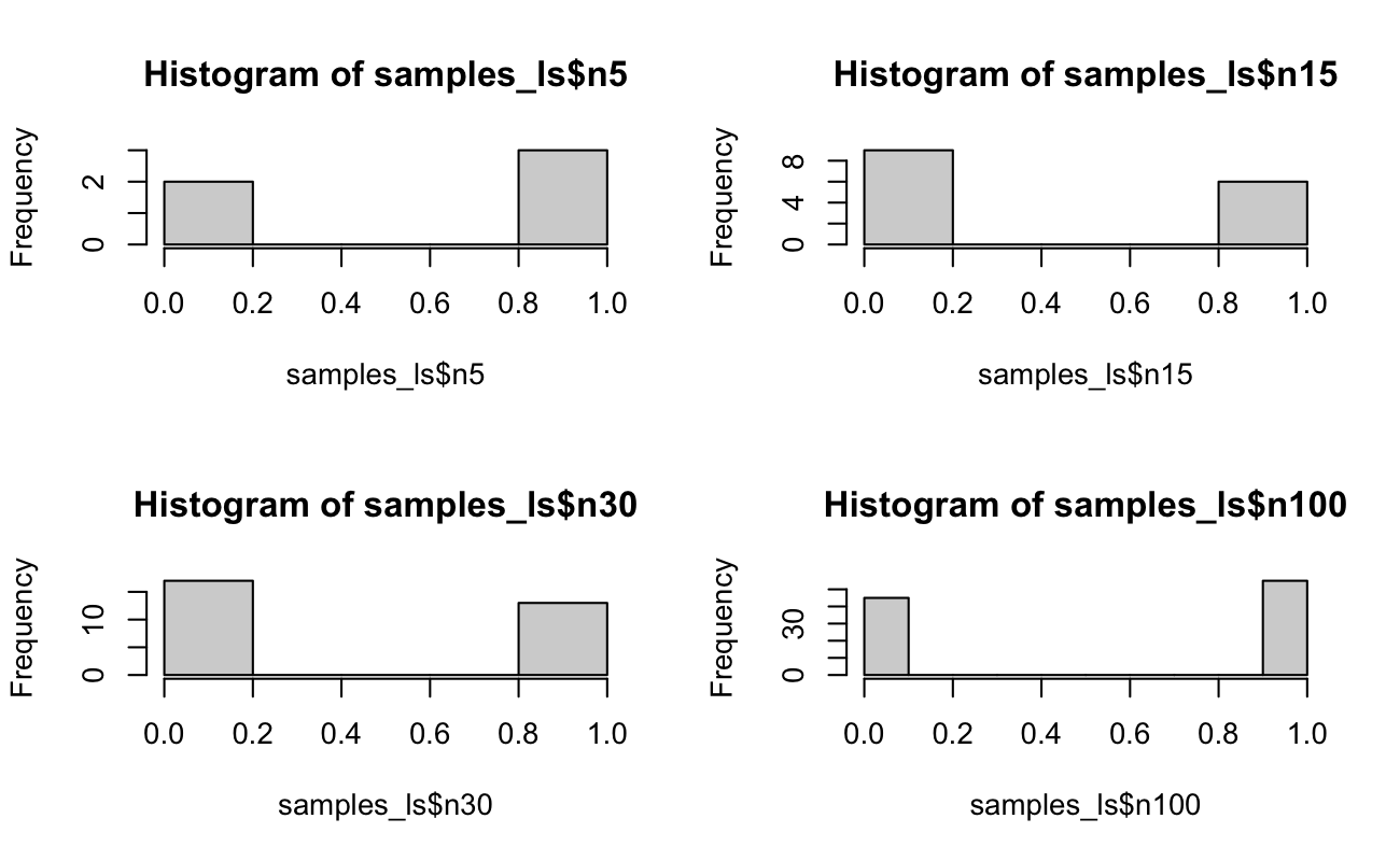

1.4 Formal Foundations

1.4.1 The Riemann-Stieltjes Integral

Let \(f\) be a bounded function on the interval \(\mathcal{S} = [a, b] \subset \mathbb{R}\)

Let \(P = \{a = x_0 < x_1 < \ldots x_k < b\}\) be the partition of \(\mathcal{S}\),

Recall the Reimann sum \(S(P,f)\) is defined as

\[ S(P,f) = \sum_\limits{i=1}^{n}f(c_i)(x_i - x_{i-1}) \] where \(c_i\) is some point in between \(x_{i-1}\) and \(x_i\), i.e. \(c_i \in [x_{i-1}, x_{i}]\)

Let \(||P|| = \max_\limits{1\le i\le n}{(x_i-x_{i-1})}\) be the mesh size.

The Reimann integral² is the limit of \(S(P,f)\) as the mesh size approaches 0:

\[ \begin{split} \int_{x \in \mathcal{S}}{f(x)dx} &= \lim_{||P|| \rightarrow 0}S(P,f) \\ &= \lim_{||P|| \rightarrow 0}\sum_\limits{i=1}^{n}f(c_i)(x_i - x_{i-1}) \end{split} \]

The main idea is that as the mesh size \(||P||\) gets smaller, the difference \((x_i - x_{i-1}) \rightarrow dx\), and \(c_i \rightarrow x\), resulting in the familiar form of the integral, which is defined geometrically as the sum over the area of rectangles with height \(f(x)\) and uniform width \(dx\) - but what if we wanted the width of those rectangles to vary as a function of x³?

Now let \(G\) be a monotone non-decreasing⁴ (but not necessarily continuous) function on \(\mathcal{S}\).

The Riemann-Stieltjes sum of \(f\) with respect to \(G\) is denoted as

\[ R\text{-}S(P,f,G) = \sum_\limits{i=1}^nf(c_i)[G(x_{i-1}) - G(x_i )] \]

And consequently the Riemann-Stieltjes integral is defined as:

\[ \begin{split} \int_{x \in \mathcal{S}}{f(x)dG(x)} &= \lim_{||P|| \rightarrow 0}R\text{-}S(P,f, G) \\ &= \lim_{||P|| \rightarrow 0}\sum_\limits{i=1}^{n}f(c_i)[G(x_i) - G(x_{i-1})] \end{split} \]

If \(G\) is continuous \(\forall x \in \mathcal{S}\), then this integral simplifies to

\[ \int_{x \in \mathcal{S}} f(x) \text{d}G(x) = \int_{x \in \mathcal{S}} f(x) G^{\prime}(x)\text{d}x. \]

If, however, there exists \(k < m < \infty\) points of discontinuity for \(G\) on \(\mathcal{S}\), we define an \(m\)-partition of \(\mathcal{S}\) as \(\{[y_0, y_1), [y_1, y_2), \ldots, [y_{m - 2}, y_{m - 1}), [y_{m - 1}, y_m]\}\), where \(\{a = y_0, b = y_m\}\) and the \(k\) points of discontinuity are included in the sequence \(\{y_1, y_2, \ldots, y_{m - 1}\}\). Then, this integral simplifies to

\[ \int_{x \in \mathcal{S}} f(x) \text{d}G(x) = \sum\limits_{i = 1}^m f(x)\left[ G(y_i) - G(y_{i - 1}) \right]. \]

By replacing \(x_i\) and \(x_{i-1}\) with \(G(x_i)\) and \(G(x_{i-1})\) respectively, we allow the width of the rectangles to vary with \(G(x)\), and because the limit is defined as sums of partitions of \(\mathcal{S}\), it is not necessary for \(G(x)\) to be differentiable everywhere for \(x\) (compared to \(dx\)). This allows statisticians to unify notation regarding discrete and continuous (and mixed) distributions⁵, by using a variable’s CDF \(F(x)\) as \(G(x)\):

\[\begin{split} \int_{x \in \mathcal{S}} f(x) \text{d}F(x) &= \sum\limits_{i = 1}^n f(x)\left[ F(x_i) - F(x_{i - 1}) \right] \\ &= \sum\limits_{i = 1}^n f(x)\left[ P(x_{i−1} < X \le x_{i}) \right] \\ &= \begin{cases} \sum_\limits{i}{f(x_i)P(X = x_i)} & \text{if } F(x) \text{ is discrete} \\ \int_{x\in\mathcal{S}}{f(x)F'(x)dx} & \text{if } F(x) \text{ is continuous} \end{cases} \end{split}\]

1.4.2 Properties of Distributions

Let \(x\) be an observed value \(\in \mathcal{A}\), and let \(\boldsymbol\theta\) be a vector of parameters in a parameter space \(\boldsymbol\Theta \subseteq \mathbb{R}^q\). Consider a function \(f(\textbf{x}|\boldsymbol\theta)\) with anti-derivative \(F\), and note that \(f\) need not be continuous. This \(f\) represents a probability distribution iff⁶

1. \(\forall x \in \mathcal{S}\), \(\forall \boldsymbol\theta \in \boldsymbol\Theta\), \(f(x|\boldsymbol\theta) \ge 0\).
2. \(\forall \boldsymbol\theta \in \boldsymbol\Theta\), \(\int_{x \in \mathcal{S}} \text{d}F(x|\boldsymbol\theta) = 1\), where \(\text{d}F\) is the integrand of a Riemann-Stieltjes integral.

As long as (1) holds above, then \(F\) will be monotone non-decreasing (because the anti-derivative of a non-negative function will always be flat or increasing). The probability density/mass functions for all statistical distributions share these two properties above. Because of the flexibility of the Riemann-Stieltjes integral, we don’t have to make the distinction between probability density functions and probability mass functions any longer. This is because

1. If \(\mathcal{S}\) is a discrete set with cardinality \(|\mathcal{S}| = n\), \(f\) is commonly referred to as a probability “mass” function. Then, because (1) holds, \(\exists\) some ordering of the elements of \(\mathcal{S} \ni 0 \le F(x^{(1)}) \le F(x^{(2)}) \le \cdots \le F(x^{(n)}) \le 1\). We know that the total probability of all events is 1, and the total probability of no events is 0, so, by convention, we let \(F(x^{(n)}) = 1\) and \(F(x^{(0)}) = 0\). Thus, noticing the Telescoping Series⁷, \[ \int_{x \in \mathcal{S}} \text{d}F(x|\boldsymbol\theta) = \sum\limits_{i = 1}^n F(x^{(i)}) - F(x^{(i - 1)}) = F(x^{(n)}) - F(x^{(0)}) = 1. \]
2. If \(\mathcal{S} = [a,b]\) is a continuous set, then \(f\) is a probability “density” function. For this continuous range, \(F(a) = 0\) and \(F(b) = 1\). Thus, \[ \int_{x \in \mathcal{S}} \text{d}F(x|\boldsymbol\theta) = \int_a^b F^{\prime}(x)dx = F(b) - F(a) = 1. \]

Thus, for the remainder of these notes, we will start all integral-based definitions with the Riemann-Stieltjes form, and then reduce this form into traditional sums or integrals, as is appropriate for the distribution at hand.

1.5 Show that this is a Distribution

Given the extensive review above, showing that \(f_{\text{Bern}}\) is a probability distribution is anti-climactic.

1.5.1 The Distribution is Non-negative

Claim: The function \(f_{\text{Bern}}\) must be non-negative for all values of its support given \(p\) in the parameter space \((0,1)\).

Argument: If \(k = 0\), then \(f_{\text{Bern}}(k = 0|p) = p^0(1 - p)^1 = 1 - p \ge 0\). Similarly, if \(k = 1\), then \(f_{\text{Bern}}(k = 1|p) = p^1(1 - p)^0 = p \ge 0\).

1.5.2 The Total Probability is 1

Claim: The integral of the function \(f_{\text{Bern}}\) over all possible values of \(k\) must be 1.

Argument: Consider that \[ \begin{aligned} \int_{x \in \mathcal{S}} \text{d}F(x|\boldsymbol\theta) &= \sum\limits_{k = 0}^1 f_{\text{Bern}}(k|p) \\ &= \left[ p^k(1-p)^{1-k} \right]_{k = 0} + \left[ p^k(1-p)^{1-k} \right]_{k = 1} \\ &= [p^0(1-p)^1] + [p^1(1-p)^0] \\ &= (1 - p) + p \\ &= 1. \end{aligned} \]

1.6 Derive the Moment Generating Function

1.6.1 Review: What is the MGF?

The Moment Generating Function⁸ (MGF) is, as its name implies, a function to “generate” (i.e., calculate) moments. In statistics, I have not found great intuition on what a “moment” is, other than it relates to various measures of a probability distribution:

• The 0\(^{\text{th}}\) moment is the total area of the probability distribution [or 1],
• The 1\(^{\text{st}}\) moment is the expected value,
• The 2\(^{\text{nd}}\) (central) moment is the variance,
• The 3\(^{\text{rd}}\) moment is the skewness, and
• The 4\(^{\text{th}}\) moment is the kurtosis.

Physics has more intuition of moments, where the 1\(^{\text{st}}\) moment is the center of mass for a body (the point at which you could balance the shape on a pencil) and the 2\(^{\text{nd}}\) moment is the moment of inertia (how much mass is spread out away from the axis at the center of mass, where larger values mean the mass is spread out further away from the first moment).

Given a Cumulative Density Function \(F_X(x|\boldsymbol\theta)\), the MGF of \(F_X\) with respect to some value \(t\) in an \(\epsilon\)-neighborhood⁹ of 0 is defined to be \[ M_X(t) \equiv \mathbb{E}\left[ e^{tX} \right] = \int\limits_{x \in \mathcal{S}(X)} e^{tx} \text{d}F_X(x|\boldsymbol\theta), \] where \(\text{d}F_X\) is the integrand of a Riemann-Stieltjes integral (as discussed above).

If we have a distribution with \(j\) parameters, the process to calculate the first \(j\) moments is to take the first \(j\) derivatives of \(M_X\) and evaluate these functions (if they exist) at \(t = 0\). Then, these theoretical moments (functions of the distribution’s parameters \(\boldsymbol\theta\)) are set equal to the first \(j = |\boldsymbol\theta|\) sample moments, yielding a system of (often non-linear) equations to solve.

1.6.2 MGF of the Bernoulli Distribution

Given the definition above, we can calculate the MGF: \[ \begin{aligned} M_K(t) &\equiv \mathbb{E}\left[ e^{tK} \right] \\ &= \int\limits_{k \in \{0,1\}} e^{tk} \text{d}F_K(k|p) \\ &= \sum\limits_{k = 0}^1 e^{tk} p^k (1 - p)^{1 - k} \\ &= \sum\limits_{k = 0}^1 (pe^t)^k (1 - p)^{1 - k} \\ &= \left[ (pe^t)^0 (1 - p)^1 \right] + \left[ (pe^t)^1 (1 - p)^0 \right] \\ &= 1 - p + pe^t. \end{aligned} \]

1.7 Method of Moments Estimators

Now that we have the MGF of the Bernoulli Distribution, we follow the process to calculate the theoretical moment(s) and set them equal to their corresponding sample moment(s). Because the Bernoulli Distribution only has \(j = 1\) parameter, our systems to solve will be somewhat trivial.

1.7.1 First Moment

Given the MGF calculated above, we begin with \[ \begin{aligned} M_K(t) &= 1 - p + pe^t \\ \Longrightarrow\qquad \frac{\partial}{\partial t}M_K(t) &= pe^t \\ \Longrightarrow\qquad \frac{\partial}{\partial t}M_K(0) &= p \\ &= \mathbb{E}[K]. \end{aligned} \]

1.7.2 The Second Moment

The second (non-central) moment is then \[ \begin{aligned} \frac{\partial}{\partial t}M_K(t) &= pe^t \\ \\ \Longrightarrow\qquad \frac{\partial^2}{\partial t^2}M_K(t) &= pe^t \\ \Longrightarrow\qquad \frac{\partial^2}{\partial t^2}M_K(0) &= p \\ &= \mathbb{E}[K^2]. \end{aligned} \]

Because this is the non-central moment, we find the second central moment by exploiting the common relationship between variance and moments; that is, \[ \begin{aligned} \text{Var}[K] &= \mathbb{E}[K^2] - \mathbb{E}^2[K] \\ &= p - [p]^2 \\ &= p(1 - p). \end{aligned} \]

1.7.3 Solving the System

For distributions with two parameters, we would now equate these two population moments, \(\mathbb{E}[K]\) and \(\text{Var}[K]\), the two sample moments, \(\bar{x}\) and \(s^2\), to yield the Method of Moments estimators for the two parameters of the distribution (which we will represent generically as \(\hat\theta_{MoM}\) and \(\hat\phi_{MoM}\)).

However, the Bernoulli has only one parameter, so our “system” of equations is just \[ \begin{aligned} \bar{x} &= p \\ \Longrightarrow \hat{p}_{MoM} &= \bar{x}. \end{aligned} \] For the data observed above, the coin-flip results \(\{\)Heads, Tails, Heads, Tails, Tails\(\}\) which came from a coin with \(P[\text{Heads}] = 0.35\), \(\hat{p}_{MoM} = \frac{1}{5}\sum_{i = 1}^5 x_i = 0.4\).

1.8 The Likelihood Function

In standard statistical inference, we assume that the population parameter is some fixed but unknown value and that our observed data are random; we must estimate the unknown (but fixed) parameter using statistics of the observed (but random) data. Likelihood functions (and the related Bayesian school of thought) turn this question “inside out”. The likelihood instead assumes that the parameter is a random variable (still unknown), but that the data are both observed and fixed.

1.8.1 Reviewing the Repeated Sampling Paradigm

Let’s recall the observed toy data: we flipped one coin five times and observed \(\{\)Heads, Tails, Heads, Tails, Tails\(\}\). Is the coin fair? Traditional statistics would say “\(p\) is unknown, but if I can collect enough data then I can estimate it with a narrow confidence interval”. In a simple coin-flip example, this is reasonable: we can hire a person to repeatedly flip that same coin for hours and hours and record the results. Eventually, we will have a sample size large enough so that we can build a confidence interval small enough to say with any requested level of “confidence” that the coin is or isn’t fair.

Recall the \((1-\alpha)\)-level confidence interval for a Bernoulli \(p\) is \[ \text{CI}(p|n,\alpha) = \hat{p} \pm \frac{z_{\alpha/2}}{\sqrt{n}}\sqrt{\hat{p}(1 - \hat{p})}, \] where \(z_{\alpha/2}\) is the Standard Normal \(z\) corresponding to the quantiles \(1 - \alpha/2\) and \(\alpha/2\). As we saw above, the true parameter value was \(p = 0.35\), which (we remark) would be impossible to know in real life.

We will assume that we take each coin flip one at a time. How many times will we have to flip the coin before the 95% CI no longer contains 0.5?

zAlpha <- qnorm(p = 0.975)
results_ls <- lapply(
  X = seq.int(from = 2, to = length(myBernSample), by = 1),
  FUN = function(n_i) {
    
    x <- myBernSample[1:n_i]
    pHat <- mean(x)
    CIwidth <- ( zAlpha / sqrt(n_i) ) * sqrt( pHat * (1 - pHat) )
    
    data.frame(
      N = n_i,
      pHat = pHat,
      CIlb = pHat - CIwidth,
      CIub = pHat + CIwidth
    )
  }
)

results_df <- do.call(rbind, results_ls)

# add trivial CI results for first coin flip
results_df <- rbind(
  data.frame(
    N = 1, pHat = myBernSample[1],
    CIlb = myBernSample[1], CIub = myBernSample[1]
  ),
  results_df
)

Let’s plot these results:

library(ggplot2)
ggplot(data = results_df) + 
  aes(x = N) +
  ylim(c(0, 1)) +
  scale_x_continuous(breaks = seq(from = 0, to = 100, by = 10)) +
  geom_abline(slope = 0, intercept = 0.5, colour = "red") + 
  geom_line(aes(y = CIlb)) + 
  geom_line(aes(y = CIub))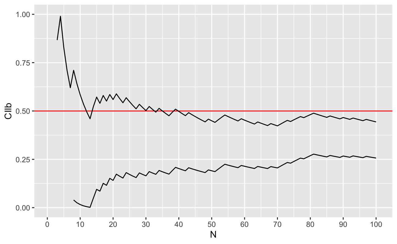

As we can see, we need between 40-45 coin flips before we can be 95% sure that the coin is “not fair” (that the true value of \(p\ne 0.5\)). Also, we see that the confidence intervals are degenerate for a few of the samples with \(n\le 5\) (that the bounds of the confidence interval for \(p\) are outside \([0,1]\), which is impossible).

1.8.2 Making the Most Use of our Data

For the computer, flipping additional coins to create new data is trivially inexpensive. However, in real life, collecting one additional sample may be of enormous cost to the research team. In these cases, it doesn’t help us that we would theoretically be able to reject the claim that \(p = 0.5\) at some point in the future (with more samples), we need to be able to make a statement about the likelihood that the coin is fair with the samples we have right now. Let the event \(\{\)Heads, Tails, Heads, Tails, Tails\(\}\) be encoded \(\textbf{x} = (1,0,1,0,0)\). Thus, we apply the multiplication rule of independent events for these five coin flips, and define the likelihood function of \(p\) given the observed data:

\[\begin{align} \mathcal{L}(p|\textbf{x}) &= \left[ p^k(1 - p)^{1 - k} \right]_{k = 1} \times \left[ p^k(1 - p)^{1 - k} \right]_{k = 0} \times \\ &\qquad \left[ p^k(1 - p)^{1 - k} \right]_{k = 1} \times \left[ p^k(1 - p)^{1 - k} \right]_{k = 0} \times \left[ p^k(1 - p)^{1 - k} \right]_{k = 0} \\ &= \left[ p^1 \right] \times \left[ (1 - p)^1 \right] \times \left[ p^1 \right] \times \left[ (1 - p)^1 \right] \times \left[ (1 - p)^1 \right] \\ &= p^2(1 - p)^3 \\ &= p^2(1 - 3p + 3p^2 - p^3) \\ &= p^2 - 3p^3 + 3p^4 - p^5. \end{align}\]

1.8.3 Integrating the Likelihood

This function \(\mathcal{L}\) contains almost all the information we have about \(p\): it has all the data, and it has our best guess about the data generating process (we think it’s a Bernoulli trial). A few things to notice:¹⁰

1. \(\mathcal{L}\) is a function of the parameter, \(p\), not of the data.
2. \(\mathcal{L}\) is NOT a probability function; even though \(\mathcal{L} \ge 0\ \forall p\), we have that the integral over the support of \(p\) is

\[\begin{align} \int_0^1 \mathcal{L}(p|\textbf{x})dp &= \int_0^1 \left[ p^2 - 3p^3 + 3p^4 - p^5 \right]dp \\ &= \frac{1}{3}p^3 - \frac{3}{4}p^4 + \frac{3}{5}p^5 - \frac{1}{6}p^6 \Big\rvert_0^1 \\ &= \frac{1}{3} - \frac{3}{4} + \frac{3}{5} - \frac{1}{6} \\ &= \frac{20}{60} - \frac{45}{60} + \frac{36}{60} - \frac{10}{60} \\ &= \frac{1}{60} \\ &\ne 1 \end{align}\]

This exercise serves two purposes: first to show that \(\mathcal{L}\) is not a probability distribution, and second to show the value of the multiplicative constant which would make a distribution. That is, \(f(p|\textbf{x}) = 60*\mathcal{L}(p|\textbf{x})\) is a probability distribution. Now we can make probabilistic statements about the value of \(p\).

We can see what the probability distribution function looks like (it should look like a Beta distribution, because it is):

p <- seq(from = 0, to = 1, length.out = 101)
f_p <- 60 * p^2 * (1 - p)^3

plot(x = p, y = f_p)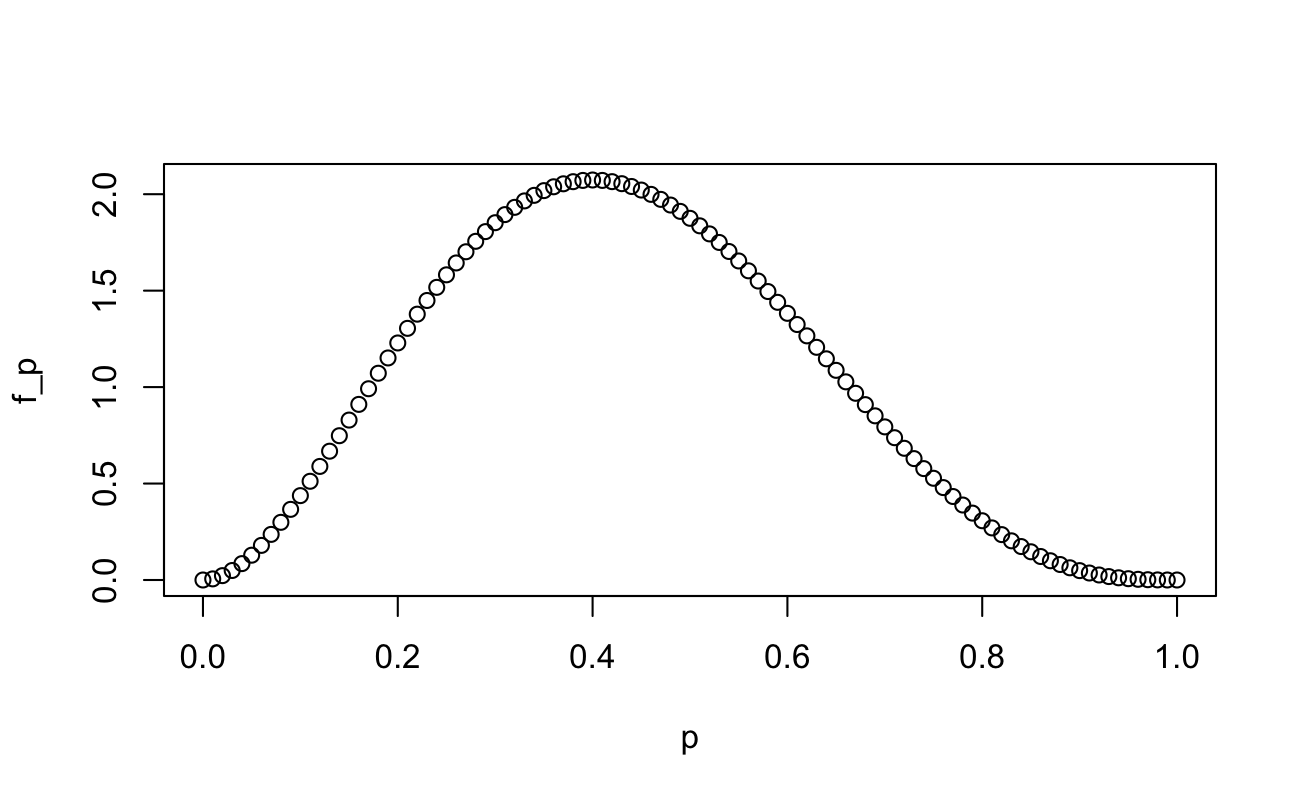

And since we have calculated the indefinite integral already, we can plot the Cumulative Distribution Function:

F_p <- 60 * (p^3/3 - 3*p^4/4 + 3*p^5/5 - p^6/6)
plot(x = p, y = F_p)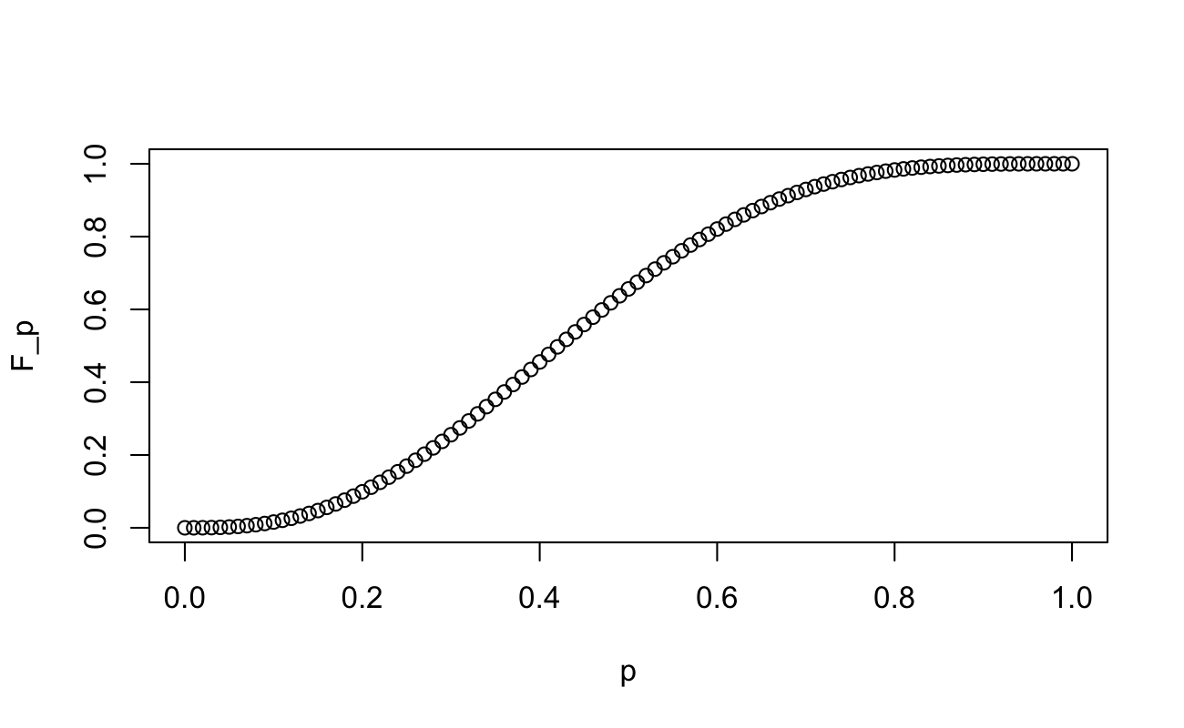

Finally, we can make statements about the claim that \(p = 0.5\). For instance, what is \(P[p < 0.5]\)?

F_p[which(p == 0.5)]
[1] 0.656

What is \(P[p > 0.5]\)?

1 - F_p[which(p == 0.5)]
[1] 0.344

What is \(P[0.4 < p < 0.6]\)?

F_p[which(p == 0.6)] - F_p[which(p == 0.4)]
[1] 0.365

What is an 80% credible set¹¹ for \(p\)?

# Lower
p[max(which(F_p < 0.1))]
[1] 0.2
# Upper
p[min(which(F_p > 0.9))]
[1] 0.67

1.9 Maximum Likelihood Estimators: The “Most Likely” Value of \(p\)

We have an integrated likelihood, which contains basically almost all there is to know about the data we’ve collected, but finding a closed form of the integral of \(\mathcal{L}\) (necessary to find \(f\) and \(F\)) can be impossible in most real-world scenarios. Rather than trying to answer all the questions about \(p\), sometimes it’s still worthwhile to answer “what is the most likely value of \(p\) given the data we’ve observed?”

This is answered with maximum likelihood estimation, and we need two steps. Using (multivariable) differential calculus, we

1. find the value of \(\boldsymbol\theta\) which maximizes \(\mathcal{L}(\boldsymbol\theta|\textbf{x})\), and
2. show that \(\mathcal{L}(\boldsymbol\theta|\textbf{x})\) is concave down¹² at this point.

For the first step, it is common practice to 1) disregard any multiplicative constants leading \(\mathcal{L}\) (because the derivative in the next step will zero these constants out) and 2) to take the natural logarithm of the likelihood and maximize that instead. Because logarithms simply change the scale of the vertical axis, they do not affect the location of extreme values. Let’s begin (I show what happens to the multiplicative constant in square brackets):

\[\begin{align} \mathcal{L}(p|\textbf{x}) &= [60\times]\ p^2(1 - p)^3,\ p\in[0,1] \\ \Longrightarrow \qquad \ell(p|\textbf{x}) &= [\log(60) +]\ 2\log(p) + 3\log(1 - p),\ p\in(0,1) \\ \Longrightarrow \qquad \frac{\partial\ell}{\partial p} &= [0+]\ \frac{2}{p} - \frac{3}{1 - p} \\ \Longrightarrow \qquad 0 &\overset{\text{set}}{=} \frac{2}{p} - \frac{3}{1 - p} \\ \Longrightarrow \qquad 0 &= 2(1 - p) - 3p \\ \Longrightarrow \qquad \hat{p} &= 2/5 \end{align}\]

The second step is to confirm that \(\hat{p} = \frac{2}{5}\) is a maximum of \(\mathcal{L}\), by ensuring that the second derivative of \(\mathcal{L}\) is negative around \(\hat{p}\). For that, we return to the first derivative of the log-likelihood (I’m using negative exponents instead of fractions because the chain rule is easier to apply than the quotient rule for these fractions), and differentiate again:

\[\begin{align} \frac{\partial\ell}{\partial p} &= 2p^{-1} - 3(1 - p)^{-1} \\ \Longrightarrow \qquad \frac{\partial^2\ell}{\partial p^2} &= -2p^{-2} + 3(1 - p)^{-2}\times(-1) \\ &= -\left( \frac{2}{p^2} + \frac{3}{(1 - p)^2} \right) <0\ \forall p \in (0,1). \end{align}\]

So, for this trivial example, both Method of Moments and Maximum Likelihood Estimation yielded the same estimate for \(\hat{p}\)¹³.

1.10 Extensions and Related Distributions

The Bernoulli distribution extends directly to the Binomial, which models the number of successes across n trials. The Multinomial generalizes this to \(k > 2\) categories, and is often used in genetics, survey sampling, and categorical data analysis. The Geometric distribution models the number of trials until the first success, while the Negative Binomial models trials until the \(r^{th}\) success or over-dispersed count data. The Poisson emerges as a limit of the binomial for rare-event incidence rates.

These models fall within the generalized linear model (GLM) framework, encompassing logit and probit models for Bernoulli outcomes and log-linear models for Poisson responses McCullagh and Nelder (2018).

In Bayesian inference, the Beta distribution serves as a conjugate prior to \(p\). Posterior updating yields \(\text{Beta}(\alpha+x, \beta+n-x)\), providing a basis for inference with binary data Gelman et al. (2013).

1.11 Exercises

1. Calculate \(E[X]\) for \(X \sim Ber(p)\) using Reimann-Stieltjes notation.

2. Derive the Geometric distribution from the Bernoulli distribution.

3. Using the dataset found in Wu et al. (2020), calculate method of moments estimators for the variables Obesity and Energy (Go to the Availability of data and materials) section to download the data.

1.12 Appendix

1.12.1 Interval Estimation

The Clopper–Pearson interval provides exact confidence bounds but is considered conservative. Approximate intervals such as the Wilson score and Agresti–Coull intervals have been shown to outperform the Wald interval by offering better coverage and shorter length. Exact methods are preferred in cases of small n or extreme counts (near 0 or n), while approximate methods are recommended for moderate-to-large n (Agresti and Coull (1998)).

Below is an example of an Agresti-Coull interval:

# x = number of successes;n = number of trials 
agrestiCoulliCI <- function(x, n, conf.level = 0.95) { 
  alpha <- 1 - conf.level 
  z <- qnorm(1 - alpha/2) 
  n_adj <- n + z^2 
  
  p_tilde <- (x + z^2/2) / n_adj 
  se <- sqrt(p_tilde * (1 - p_tilde) / n_adj) 
  
  lower <- p_tilde - z * se 
  upper <- p_tilde + z * se
  
  return(c(lower = max(0, lower), 
           estimate = p_tilde, 
           upper = min(1, upper))) 
  } 

# Example: 45 successes out of 100 trials agresti_coull_ci(x = 45, n = 100, conf.level = 0.95)


agrestiCoulliCI(2, 5)
   lower estimate    upper 
   0.116    0.443    0.771 

1.12.2 Hypothesis Testing

One-sample tests for \(p\) include the exact binomial test and large-sample normal approximations. Two-sample tests compare proportions using score or chi-square methods, while Fisher’s exact test is appropriate for small samples and sparse tables. These approaches are commonplace in applied biostatistics and epidemiology for treatment/control comparisons and case-control studies.

1.12.3 Inference Properties

Sufficient statistic \(T = \sum_\limits{i=1}^n{X_i}\) is complete, so by the Lehmann–Scheffe theorem, \(\hat{p}\) is the uniformly minimum variance unbiased estimator (UMVUE). Its variance attains the Cramér–Rao lower bound, demonstrating efficiency.

1.13 Footnotes

Abbasi, Azhar Mehmood, Muhammad Yousaf Shad, and Aneel Ahmed. 2022. “On Partial Randomized Response Model Using Ranked Set Sampling.” PLOS ONE 17 (11): e0277497. https://doi.org/10.1371/journal.pone.0277497.

Agegnehu, Chilot Desta, and Adugnaw Zeleke Alem. 2021. “Exploring Spatial Variation in BCG Vaccination Among Children 0–35 Months in Ethiopia: Spatial Analysis of Ethiopian Demographic and Health Survey 2016.” BMJ Open 11 (4): e043565. https://doi.org/10.1136/bmjopen-2020-043565.

Agresti, Alan, and Brent A. Coull. 1998. “Approximate Is Better Than ‘Exact’ for Interval Estimation of Binomial Proportions.” The American Statistician 52 (2): 119–26. https://doi.org/10.1080/00031305.1998.10480550.

Branson, Zach, and Marie-Abèle Bind. 2019. “Randomization-Based Inference for Bernoulli Trial Experiments and Implications for Observational Studies.” Statistical Methods in Medical Research 28 (5): 1378–98. https://doi.org/10.1177/0962280218756689.

Gelman, Andrew, John B. Carlin, Hal S. Stern, David B. Dunson, Aki Vehtari, and Donald B. Rubin. 2013. Bayesian Data Analysis. 3rd ed. Chapman & Hall/CRC.

Hosmer, David W., Stanley Lemeshow, and Rodney X. Sturdivant. 2013. Applied Logistic Regression. 3rd ed. Wiley.

Johnson, Norman L., Adrienne W. Kemp, and Samuel Kotz. 2005. Univariate Discrete Distributions. 3rd ed. Wiley. https://onlinelibrary.wiley.com/doi/book/10.1002/0471715816.

McCullagh, P., and John A. Nelder. 2018. Generalized Linear Models. Boca Raton: Chapman; Hall/CRC.

Thompson, E. A. 2010. “Minimum Variance Estimators.” https://faculty.washington.edu/eathomp/S341_10/Hwks/Cramer_Rao_soln.pdf.

Wu, Bangsheng, Yi Jiang, Xiaoqing Jin, and Li He. 2020. “Using Three Statistical Methods to Analyze the Association Between Exposure to 9 Compounds and Obesity in Children and Adolescents: NHANES 2005-2010.” Environmental Health 19 (1): 94. https://doi.org/10.1186/s12940-020-00642-6.

Xue, Xiaonan, and Ron Brookmeyer. 1997. “Regression Analysis of Discrete Time Survival Data Under Heterogeneity.” Statistics in Medicine 16 (17): 1983–93. https://doi.org/10.1002/(SICI)1097-0258(19970915)16:17<1983::AID-SIM628>3.0.CO;2-3.

---

1. https://www.usu.edu/math/schneit/StatsStuff/Probability/probability2.html

2. https://en.wikipedia.org/wiki/Riemann_integral

3. A good video on visualizing the RS Integral

4. Some texts will say monotone increasing, which is a more strict requirement. However, the functions we will apply this to are all cumulative density functions, so they are (mostly) well-behaved. Thus, we can have the slightly less restrictive condition of monotone non-decreasing.

5. Another good video on the derivation specifically for statisticians

6. if and only if

7. https://en.wikipedia.org/wiki/Telescoping_series

8. https://en.wikipedia.org/wiki/Moment-generating_function

9. \(t \in (-\epsilon, \epsilon) \subset \mathbb{R}\) (where \(\epsilon\) is an arbitrarily small value)

10. We could also notice that this is the kernel of a Beta distribution with \(\alpha = 3\) and \(\beta = 4\), with normalizing constant \(\frac{(3-1)!(4-1)!}{(3+4-1)!} = \frac{2}{6*5*4} = \frac{1}{60}\), but that would make the next steps too easy…

11. https://en.wikipedia.org/wiki/Credible_interval

12. https://tutorial.math.lamar.edu/classes/calci/shapeofgraphptii.aspx

13. This estimator is unbiased with variance \(Var(\hat{p})=\frac{p(1-p)}{n}\) and achieves the Cramér–Rao lower bound, making it efficient under standard MLE conditions Thompson (2010)