As with the chapter on the Student’s \(t\) distribution, we will not include sections on the Method of Moments or Maximum Likelihood Estimators. Also, before we move on, please review the definition of the \(\chi^2\) Distribution from that chapter. We begin by letting \(X \sim \chi^2_{\nu_x}\) and \(Y \sim \chi^2_{\nu_y}\) and by assuming that \(X \perp Y\). The joint distribution of \(X\) and \(Y\) is \[
f_{X,Y}(x,y|\nu_x, \nu_y) = \left[ \frac{2^{-\frac{\nu_x}{2}}}{\Gamma\left(\frac{\nu_x}{2}\right)} x^{\frac{\nu_x}{2} - 1} e^{-\frac{x}{2}} \right] \left[ \frac{2^{-\frac{\nu_y}{2}}}{\Gamma\left(\frac{\nu_y}{2}\right)} y^{\frac{\nu_y}{2} - 1} e^{-\frac{y}{2}} \right].
\]
Similarly to our work on the Student’s \(t\) Distribution, we will make a creative bivariate substitution. Let \(G = Y\) be the nuisance parameter, and let \[
H = \frac{X/\nu_x}{Y/\nu_y} \Rightarrow \frac{Y}{\nu_y}H = \frac{X}{\nu_x} \Rightarrow \frac{\nu_x}{\nu_y}GH = X.
\] For the support of these variables, recall that \(X,Y > 0\), so \(H,G > 0\). For this substitution, the Jacobian Determinant is found by \[
\begin{aligned}
\textbf{J} &= \begin{bmatrix}
\frac{\partial X}{\partial H} & \frac{\partial Y}{\partial H} \\
\frac{\partial X}{\partial G} & \frac{\partial Y}{\partial G} \\
\end{bmatrix} \\
&= \begin{bmatrix}
\frac{\partial}{\partial H} \frac{\nu_x}{\nu_y}GH & \frac{\partial}{\partial H} G \\
\frac{\partial}{\partial G} \frac{\nu_x}{\nu_y}GH & \frac{\partial}{\partial G} G \\
\end{bmatrix} \\
&= \begin{bmatrix}
\frac{\nu_x}{\nu_y}G & 0 \\
\frac{\nu_x}{\nu_y}H & 1 \\
\end{bmatrix} \\
\Longrightarrow \det(\textbf{J}) &= \frac{\nu_x}{\nu_y}G(1) - (0)\frac{\nu_x}{\nu_y}H \\
&= \frac{\nu_x}{\nu_y}G.
\end{aligned}
\]
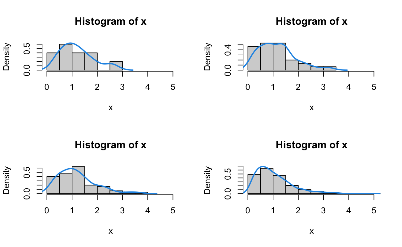
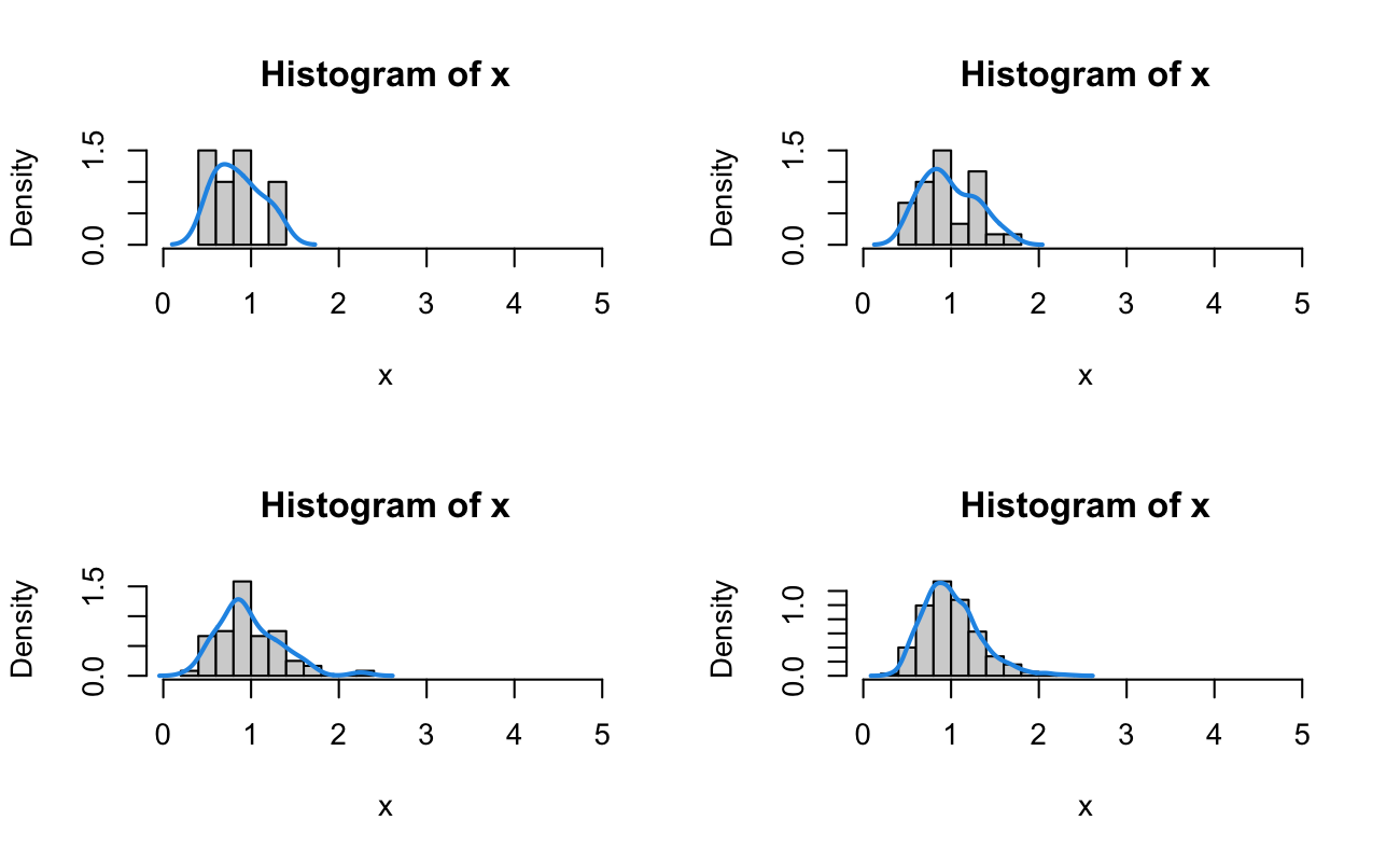
set.seed(20150516)# F for a well-posed linear model [p = 5, n = 100]xWP <-rf(n =1000, df1 =4, df2 =99)samplesWP_ls <-list(n10 = xWP[1:10],n30 = xWP[1:30],n60 = xWP[1:60],n1000 = xWP)# F for a poorly-posed linear model [p = 25, n = 100]xPP <-rf(n =1000, df1 =24, df2 =99)samplesPP_ls <-list(n10 = xPP[1:10],n30 = xPP[1:30],n60 = xPP[1:60],n1000 = xPP)range_num <-range(c(xWP, xPP))rm(xWP, xPP)
We will change the notation a tiny bit (using \(x\) as our random variable instead of \(h\)). Here is our Central \(\mathcal{F}\) Distribution with \(\nu_1, \nu_2\) degrees of freedom: \[
f_{\mathcal{F}}(x|\nu_1,\nu_2) = \frac{ \Gamma\left( \frac{\nu_1 + \nu_2}{2} \right) }{ \Gamma\left(\frac{\nu_1}{2}\right) \Gamma\left(\frac{\nu_2}{2}\right) } \left[\frac{\nu_1}{\nu_2}\right]^{\frac{\nu_1}{2}} \frac{ x^{\frac{\nu_1}{2} - 1} }{ \left( \frac{\nu_1}{\nu_2}x + 1 \right)^{\frac{\nu_1 + \nu_2}{2}} }.
\] Because these degrees of freedom parameters are counts of independent pieces of information, we have the restriction that \(\nu_1,\nu_2 > 0\). Also, based on the change of variables we employed above, \(x > 0\). By these two restrictions, \[
\begin{aligned}
\frac{ \Gamma\left( \frac{\nu_1 + \nu_2}{2} \right) }{ \Gamma\left(\frac{\nu_1}{2}\right) \Gamma\left(\frac{\nu_2}{2}\right) } &> 0, \\
\frac{\nu_1}{\nu_2} &> 0,\ \text{and} \\
\frac{\nu_1}{\nu_2}x + 1 &> 0;\ \text{so} \\
\frac{ x^{\frac{\nu_1}{2} - 1} }{ \left( \frac{\nu_1}{\nu_2}x + 1 \right)^{\frac{\nu_1 + \nu_2}{2}} } &> 0.
\end{aligned}
\] Hence \(f_{\mathcal{F}} > 0\) for \(x,\nu_1,\nu_2 > 0\).