We will begin this lesson a little differently. For the previous lessons, we were able to derive the distributions without a tremendous amount of preliminary mathematics. However, while the Poisson distribution will end up as a simple distribution to work with, deriving it requires a deep refresh of calculus in addition to some of the other Formal Foundations we have already seen.
4.1.1 The Limit Definition of the Derivative
In our introductory calculus courses, we first learned that the derivative was a sophisticated “slope” of a function. Consider some function \(y = f(x)\) and its first derivative, which is most commonly denoted as \(y^{\prime}\), \(f^{\prime}(x)\), or \(\frac{dy}{dx}\). Specifically, we learned that \(f^{\prime}(x)\) is the function that yields the instantaneous rate of change of the function \(f(x)\). That is, the function \(f\) at the point \(x = x_0\) is parallel to every straight line which has a slope given by the value of the function \(f^{\prime}(x)\) evaluated at \(x = x_0\).
In the above picture (from the engineers at Utah State University), the red curve is the function \(f(x)\), the evaluation point is the black dot near \(\{x = 2.25,\ y = 1.25\}\), and the blue line is the tangent line1 to \(f(x)\) at the evaluation point. It’s the line that has a slope given by \(f^{\prime}\) evaluated at the black dot.
In basic algebra, we know that we calculate the slope between two points, \(\{x,y\}\) and \(\{x_0,y_0\}\), as “the change in \(y\) divided by the change in \(x\)”. We use \(\Delta y\) to represent the “change in \(y\)”, and \(\Delta x\) similarly for \(x\). Let’s begin there, noting that \(\{x_0,y_0\} = \{x + \Delta x,y + \Delta y\}\): \[
\begin{aligned}
\text{Slope} &= \frac{y_0 - y}{x_0 - x} \\
&= \frac{f(x_0) - f(x)}{x_0 - x}\\
&= \frac{f([x + \Delta x]) - f(x)}{[x + \Delta x] - x} \\
&= \frac{f(x + \Delta x) - f(x)}{\Delta x}.
\end{aligned}
\] Given two fixed points, \(\{x,y\}\) and \(\{x_0,y_0\}\), these ratio above can be calculated directly. However, we said above that the derivative is called the instantaneous rate of change. That means, we want \(\{x,y\}\) and \(\{x_0,y_0\}\) to be “infinitely” close to each other. In other words, we want \(\Delta x \rightarrow 0\). This yields our well-known limit definition of the derivative2: \[
f^{\prime}(x) \equiv \lim_{\Delta x \rightarrow 0} \frac{f(x + \Delta x) - f(x)}{\Delta x}.
\] This limit calculation yields the first order derivative3 if we take it only once (but higher order derivatives can be found by sequentially repeating this process).
For example, the first order derivative of \(y = x^2\) via limit definition is \[
\begin{aligned}
y^{\prime} &= \lim_{\Delta x \rightarrow 0} \frac{f(x + \Delta x) - f(x)}{\Delta x} \\
&= \lim_{\Delta x \rightarrow 0} \frac{\left[ (x + \Delta x)^2 \right] - \left[ x^2 \right]}{\Delta x} \\
&= \lim_{\Delta x \rightarrow 0} \frac{x^2 + 2x\Delta x + (\Delta x)^2 - x^2}{\Delta x} \\
&= \lim_{\Delta x \rightarrow 0} \frac{\Delta x(2x + \Delta x)}{\Delta x} \\
&= \lim_{\Delta x \rightarrow 0} 2x + \Delta x \\
&= 2x + 0,
\end{aligned}
\] which is the well-known first-order derivative of \(y = x^2\) with respect to \(x\).
4.1.2 Homogeneous Functions
A function \(f(x)\) is said to be homogeneous4 iff \(f(c\textbf{x}) = c^kf(\textbf{x})\) for some scalar \(c\) and \(k \in \mathbb{N}\). The value of \(k\) in the equation is known as the “degree of homogeneity” (which isn’t super important for us to know, but I digress), but it must be an integer. What’s important about homogeneous functions is that they are stretched (but aren’t “shifted”) in space: \(f(\textbf{x})\) and \(c^kf(\textbf{x})\) all have “zeroes” at the same values of the vector \(\textbf{x}\). These functions are often sums or products of single-term polynomials.
For example, consider \(f(x,y) = x^3 + y^3\). If I pick an arbitrary constant, say 10, then \[
f(10x, 10y) = (10x)^3 + (10y)^3 = 10^3(x^3 + y^3) = 10^kf(x,y),
\] with \(k = 3\). Thus \(f(x) = x^3\) is homogeneous with degree 3. In contrast, consider the counter-example \(f(x) = x^2 - 3\). For that same arbitrary constant above, is \(f(10x)\) the same as some power of 10 times \(f(x)\)? Well, \(f(10x) = 10^2x^2 + 3 = 10^2(x^2 + \frac{3}{100}) \ne 10^k f(x)\). So \(f(x) = x^2 - 3\) is not homogeneous. As another counter-example, consider \(f(x,y) = x^2 + y\). We see that \[
f(10x, 10y) = 10^2x^2 - 10y = 10^2(x^2 - \frac{1}{10}y) \ne 10^kf(x,y).
\] You may have forgotten about homogeneous functions because of how limiting they are. However, they play a very important role in solving differential equations.
Now that we understand what a first order derivative and a homogeneous function are, we can find out what the build up was all about. Differential Equations are mathematical expressions that systematically equate unknown functions and their derivatives. A primer on solving ordinary5 differential equations is well beyond the scope of this material. However, we can review a very small collection of ordinary differential equations, known as homogeneous first order differential equations which have the form \[
M(x,y) + N(x,y)\frac{dy}{dx} = 0,
\] where \(M\) and \(N\) are both homogeneous functions of the same degree \(n\). Because these two functions are homogenous with the same degree \(n\), then we can write this derivative as a function of \(\frac{y}{x}\). That is, \[
\begin{aligned}
0 &= M(x,y) + N(x,y)\frac{dy}{dx} \\
\Longrightarrow \frac{dy}{dx} &= -\frac{M(x,y)}{N(x,y)} \\
\Longrightarrow \frac{dy}{dx} &= -f\left(\frac{y}{x}\right),
\end{aligned}
\] for some function \(f\). Now, we can substitute \(y = ux\) on both sides, and distribute the derivative through the substitution with the product rule. Thus, we can separate6 this differential equation into two independent functions of \(x\) and \(u\): \[
\begin{aligned}
\frac{dy}{dx} &= -f\left(\frac{y}{x}\right) \\
\Longrightarrow \frac{d(ux)}{dx} &= -f\left(\frac{ux}{x}\right) \\
\Longrightarrow u\frac{dx}{dx} + x\frac{du}{dx} &= -f(u) \\
\Longrightarrow x\frac{du}{dx} &= -f(u) - u \\
\Longrightarrow \frac{1}{x}\frac{dx}{du} &= \frac{-1}{f(u) + u} \\
\Longrightarrow \int \frac{1}{x}dx &= \int \frac{-1}{f(u) + u}du,
\end{aligned}
\] which can be solved if the integral of the right hand side can be found. We note that the solution to the left hand side is \(\ln(x)\).
Let’s have an example before we move on (we’ll work something similar to this example from Newcastle University). Consider \[
\begin{aligned}
(x^2 + y^2) + x^2\frac{dy}{dx} &= 0 \\
\Longrightarrow \frac{dy}{dx} &= -\frac{x^2 + y^2}{x^2} \\
\Longrightarrow \frac{dy}{dx} &= -1 - \left(\frac{y}{x}\right)^2.
\end{aligned}
\] Now, we let \(y = ux\), so \(\frac{dy}{dx} = u + x\frac{du}{dx}\). Hence, \[
\begin{aligned}
\frac{dy}{dx} &= -\left(\frac{y}{x}\right)^2 - 1 \\
\Longrightarrow u + x\frac{du}{dx} &= -u^2 - 1 \\
\Longrightarrow x\frac{du}{dx} &= -u^2 -u - 1 \\
\Longrightarrow \frac{1}{x}dx &= -\frac{1}{u^2 + u + 1}du \\
&= -\frac{1}{\left[u^2 + u + \frac{1}{4}\right] + \left[1 - \frac{1}{4}\right]}du \\
&= -\frac{1}{ \left[u + \frac{1}{2}\right]^2 + \left[ \frac{\sqrt{3}}{2} \right]^2 }du \\
&= -\frac{\frac{4}{3}}{ \left[\frac{2}{\sqrt{3}}\left(u + \frac{1}{2}\right)\right]^2 + \frac{4}{3}\left[ \frac{\sqrt{3}}{2} \right]^2 }du \\
&= -\frac{4}{3} \frac{1}{ \left[\frac{1}{\sqrt{3}}\left(2u + 1\right)\right]^2 + 1 }du.
\end{aligned}
\]
While the last few lines may have seemed bizarre, unintuitive, and adding needless complexity, there is a method to our madness. It is known that7\[
\arctan(x) \equiv \int \frac{1}{x^2 + 1}dx.
\] Therefore, substituting \(a = \frac{1}{\sqrt{3}}(2u + 1)\) so that \(da = \frac{2}{\sqrt{3}}du\), \[
\begin{aligned}
\frac{1}{x}dx &= -\frac{4}{3} \frac{1}{ \left[ \frac{1}{\sqrt{3}} (2u + 1) \right]^2 + 1 }du \\
\Longrightarrow \int \frac{1}{x}dx &= -\frac{4}{3} \int \frac{1}{a^2 + 1} \left( \frac{\sqrt{3}}{2}da \right) \\
\Longrightarrow \ln(x) &= -\left[ \frac{4}{3}\frac{\sqrt{3}}{2} \right] \arctan\left(\frac{1}{\sqrt{3}}(2u + 1)\right) + C \\
&= -\frac{2}{\sqrt{3}} \arctan\left( \frac{2}{\sqrt{3}}\left[\frac{y}{x}\right] + \frac{1}{\sqrt{3}} \right) + C,
\end{aligned}
\] where \(C\) is the integrating constant8, which can be solved for in cases where an initial value9 is known. We will solve for \(C\) below while deriving the Poisson Distribution, so we will discuss that in more detail later.
Now, if solving this differential equation was miserable for you, take solace in knowing that we just solved the most challenging one that we will need to tackle in this course. If you had fun solving this integral, I suggest you take more electives in the mathematics department during your graduate work.
4.1.4 Integrating Factors
When we have a linear10 first order differential equation, there are various techniques and strategies that work based on the form of the differential equation. When we have a differential equation with the form \[
\frac{dy}{dx} + yf(x) = g(x),
\] then we can multiply both sides of the equation by an integrating factor11 to make the problem easier to solve. Recall the Product Rule: \[
\frac{d}{dx}\left[f(x) \times g(x)\right] \equiv f(x) \frac{dg}{dx} + g(x) \frac{df}{dx}
\] So the purpose of the integrating factor is to find something that can be multiplied by the differential equation so that the left hand can be re-written as the derivative of a product.
For differential equations in the form above, the well-known integrating factor is \[
I(x) = \exp\left[ \int f(x)dx \right].
\] Let’s confirm this via algebraic manipulation, starting with the product rule form of \(y \times I(x)\), then invoking the chain rule on \(I(x)\): \[
\begin{aligned}
\frac{d}{dx} \left( y \times I(x) \right) &= \frac{d}{dx} \left( y \times \exp\left[ \int f(x)dx \right] \right) \\
&= y \times \left( \frac{d}{dx} \exp\left[ \int f(x)dx \right] \right) + \exp\left[ \int f(x)dx \right] \frac{dy}{dx} \\
&= y \left( \exp\left[ \int f(x)dx \right] \right) \frac{d}{dx} \int f(x)dx + \exp\left[ \int f(x)dx \right] \frac{dy}{dx} \\
&= yf(x) \exp\left[ \int f(x)dx \right] + \exp\left[ \int f(x)dx \right] \frac{dy}{dx} \\
&= \exp\left[ \int f(x)dx \right] \left( \frac{dy}{dx} + yf(x) \right).
\end{aligned}
\]
Now, using what we know, we substitute this into the original differential equation: \[
\begin{aligned}
\frac{dy}{dx} + yf(x) &= g(x) \\
\Longrightarrow \exp\left[ \int f(x)dx \right] \left( \frac{dy}{dx} + yf(x) \right) &= g(x) \exp\left[ \int f(x)dx \right] \\
\Longrightarrow \frac{d}{dx} \left( y \times \exp\left[ \int f(x)dx \right] \right) &= g(x) \exp\left[ \int f(x)dx \right] \\
\Longrightarrow y\exp\left[ \int f(x)dx \right] &= \int g(x) \exp\left[ \int f(x)dx \right] dx,
\end{aligned}
\] which can often be solved, or at least simplified, if \(f(x)\) is a “nice” function.
4.2 Deriving the Distribution
Now that we have recalled the basics of very simple solving ordinary differential equations, we can follow along with Prof. Cowen’s notes on deriving the Poisson distribution.12 Suppose we are counting independent events which happen over a fixed interval of time (such as patients visiting a clinic each hour). Let \(t\) be the time, let \(\{T, T + \Delta t\}\) be a finite interval of time with width \(\Delta t\), and let \(1\) indicate that the event occurs within the interval (for example, that a single patient enters the clinic within this next small window of time). Then, we can express the probability of a new event happening between “now” (time \(T\)) and the next \(\Delta t\) few seconds as \[
\mathbb{P}\left[1 | T \le t \le T + \Delta t \right] = \lambda \Delta t,
\] where \(\lambda\) is the “rate” of visits within a standard “unit” of time (like an hour). We can then see that this product \(\lambda \Delta t\) is the rate over an hour (\(\lambda\)) multiplied by the amount of time in our small observation interval (\(\Delta t\)). Because “now” (time \(T\) is arbitrary), we simplify this notation a bit and say \[
\begin{aligned}
\mathbb{P}(1|\Delta t) &\equiv \lambda \Delta t \\
\mathbb{P}(0|\Delta t) &\equiv 1 - \lambda \Delta t.
\end{aligned}
\] Finally, let’s assume that we already know if an event occurred before “now”. That is, \(\mathbb{P}[0|t \le T]\) and \(\mathbb{P}[1|t \le T]\) are known.
4.2.1 Probability that the First Event will Happen Later
Because events are independent, the probability that the “first” event happens after the next \(\Delta t\) (that no events have happened yet AND no events will happen for the next \(\Delta t\) units of time) is \[
\begin{aligned}
\mathbb{P}(0|\Delta t) &\equiv \mathbb{P}(0|t \le T + \Delta t) \\
&= \mathbb{P}(0|t \le T) \times \mathbb{P}(0|T \le t \le T + \Delta t) \\
&= \mathbb{P}(0|t \le T) \times (1 - \lambda \Delta t) \\
&= \mathbb{P}(0|t \le T) - \lambda \mathbb{P}(0|t \le T) \Delta t \\
\Longrightarrow \mathbb{P}(0|t \le T + \Delta t) - \mathbb{P}(0|t \le T) &= - \lambda \mathbb{P}(0|t \le T) \Delta t \\
\Longrightarrow \frac{\mathbb{P}(0|t \le T + \Delta t) - \mathbb{P}(0|t \le T)}{\Delta t} &= - \lambda \mathbb{P}(0|t \le T).
\end{aligned}
\]
Notice that we are interested in the “instantaneous” probability of the next event. Hence, we want to take \(\Delta t \rightarrow 0\), which will yield a first order, linear differential equation. Thus, \[
\begin{aligned}
\frac{\mathbb{P}(0|t \le T + \Delta t) - \mathbb{P}(0|t \le T)}{\Delta t} &= - \lambda \mathbb{P}(0|t \le T) \\
\Longrightarrow \lim_{\Delta t \rightarrow 0} \frac{\mathbb{P}(0|t \le T + \Delta t) - \mathbb{P}(0|t \le T)}{\Delta t} &= - \lim_{\Delta t \rightarrow 0} \lambda \mathbb{P}(0|t \le T) \\
\Longrightarrow \frac{d}{dt} \mathbb{P}(0|t \le T) &= - \lambda \mathbb{P}(0|t \le T) \\
\Longrightarrow \frac{1}{\mathbb{P}(0|t \le T)} d\mathbb{P}(0|t \le T) &= - \lambda dt \\
\Longrightarrow \int \frac{1}{\mathbb{P}(0|t \le T)} d\mathbb{P}(0|t \le T) &= -\lambda \int dt \\
\Longrightarrow \ln\left[ \mathbb{P}(0|t \le T) \right] &= - \lambda t + C \\
\Longrightarrow \mathbb{P}(0|t \le T) &= e^{-\lambda t + C} \\
&= Ae^{-\lambda t},
\end{aligned}
\] for some constant \(A\).
Now, we have the general solution, but we can incorporate the initial condition that \(\mathbb{P}(0|t = 0) = 1\); that is, that no successes occurred before the experiment started. In our example of clinic visits, this means that no patients were already hiding inside the clinic before the doors opened in the morning. Therefore, we have that \(Ae^{-\lambda (0)} = 1\), so \(A = 1\). Therefore, \[
\mathbb{P}(0|t \le T) = e^{-\lambda t}.
\] This is the answer to the question: “what is the probability we haven’t seen the first event yet and won’t see the first event right now?”
4.2.2 A General Form for the Probability of \(n\) Events So Far
The next question we must answer to derive this distribution is: “what is the probability that we will have observed \(n\) events right now?” Or, \(\mathbb{P}(n|t \le T + \Delta t)\)? We first assume that \(\Delta t\) is small enough that multiple events cannot occur simultaneously; mathematically, we say \(\Delta t \in (0,\epsilon)\) for sufficiently small \(\epsilon\). This is a composite of two possibilities:
All \(n\) events have already happened AND we will not observe an event “now”; that is, \(\mathbb{P}(n|t \le T) \times \mathbb{P}(0|T \le t \le \Delta t)\), which we represent in shorthand as \(\mathbb{P}(n|T)\mathbb{P}(0|\Delta t)\).
All but 1 event has already happened AND we will observe an event “now”; that is, \(\mathbb{P}(n - 1|t \le T) \times \mathbb{P}(1|T \le t \le \Delta t)\), which we represent in shorthand as \(\mathbb{P}(n - 1|T)\mathbb{P}(1|\Delta t)\).
Recall that we defined \(\mathbb{P}(1|\Delta t) \equiv \lambda \Delta t\) and \(\mathbb{P}(0|\Delta t) \equiv 1 - \lambda \Delta t\). Thus (using our shorthand notation to move from the first to the second line), \[
\begin{aligned}
\mathbb{P}(n|t \le T + \Delta t) &= \mathbb{P}(n|t \le T) \times \mathbb{P}(0|T \le t \le \Delta t) + \mathbb{P}(n - 1|t \le T) \times \mathbb{P}(1|T \le t \le \Delta t) \\
\Longrightarrow \mathbb{P}(n|T + \Delta t) &= \mathbb{P}(n|T) \mathbb{P}(0|\Delta t) + \mathbb{P}(n - 1|T) \mathbb{P}(1|\Delta t) \\
&= \mathbb{P}(n|T) \left[ 1 - \lambda \Delta t \right] + \mathbb{P}(n - 1|T) \left[ \lambda \Delta t \right] \\
&= \mathbb{P}(n|T) - \lambda \mathbb{P}(n|T) \Delta t + \lambda \mathbb{P}(n - 1|T) \Delta t.
\end{aligned}
\]
Now, we will follow a similar strategy as above. We will first rearrange terms, then construct a derivative as we take \(\Delta t \rightarrow 0\), and finally identify the components of the differential equation which yield an Integrating Factor. Thus, \[
\begin{aligned}
\mathbb{P}(n|T + \Delta t) - \mathbb{P}(n|T) + \lambda \mathbb{P}(n|T) \Delta t &= \lambda \mathbb{P}(n - 1|T) \Delta t \\
\Longrightarrow \frac{\mathbb{P}(n|T + \Delta t) - \mathbb{P}(n|T)}{\Delta t} + \lambda \mathbb{P}(n|T) &= \lambda \mathbb{P}(n - 1|T) \\
\Longrightarrow \lim_{\Delta t \rightarrow 0} \frac{\mathbb{P}(n|T + \Delta t) - \mathbb{P}(n|T)}{\Delta t} + \lambda \mathbb{P}(n|T) &= \lim_{\Delta t \rightarrow 0} \lambda \mathbb{P}(n - 1|T) \\
\Longrightarrow \frac{d}{dt} \mathbb{P}(n|T) + \lambda \mathbb{P}(n|T) &= \lambda \mathbb{P}(n - 1|T),
\end{aligned}
\] so for the Integrating Factor, \(f(x) = \lambda\) and \(g(x) = \lambda \mathbb{P}(n - 1|T)\). Therefore, \(I(x) = \exp\left[\int\lambda dt\right]\), and \[
\begin{aligned}
\frac{d}{dt} \mathbb{P}(n|T) + \lambda \mathbb{P}(n|T) &= \lambda \mathbb{P}(n - 1|T) \\
\Longrightarrow \exp\left[\int\lambda dt\right] \times \left( \frac{d}{dt} \mathbb{P}(n|T) + \lambda \mathbb{P}(n|T) \right) &= \exp\left[\int\lambda dt\right] \times \lambda \mathbb{P}(n - 1|T) \\
\Longrightarrow e^{\lambda t + C} \times \left( \frac{d}{dt} \mathbb{P}(n|T) + \lambda \mathbb{P}(n|T) \right) &= e^{\lambda t + C} \times \lambda \mathbb{P}(n - 1|T) \\
\Longrightarrow e^{\lambda t} \times \left( \frac{d}{dt} \mathbb{P}(n|T) + \lambda \mathbb{P}(n|T) \right) &= e^{\lambda t} \times \lambda \mathbb{P}(n - 1|T) \\
\Longrightarrow \frac{d}{dt} \left( e^{\lambda t} \mathbb{P}(n|T) \right) &= \lambda e^{\lambda t} \mathbb{P}(n - 1|T).
\end{aligned}
\]
While this is a solution, we don’t know how to integrate \(\mathbb{P}(n - 1|T)\) for any arbitrary \(n\).
4.2.3 A Closed Form of the Distribution for Small \(n\)
Even though the general solution we found above isn’t particularly helpful for a specific value of \(n\), we do have a closed form for \(n = 0\). We showed that \(\mathbb{P}(0|T) = e^{-\lambda t}\) in the first derivation subsection. Therefore, we will leave this solution still in the form of a differential equation and construct the equations iteratively for all \(n\). We start with \(n = 1\): \[
\begin{aligned}
\frac{d}{dt} \left( e^{\lambda t} \mathbb{P}(n|T) \right) &= \lambda e^{\lambda t} \mathbb{P}(n - 1|T) \\
\Longrightarrow \frac{d}{dt} \left( e^{\lambda t} \mathbb{P}(n = 1|T) \right) &= \lambda e^{\lambda t} \mathbb{P}(n - 1 = 0|T) \\
&= \lambda e^{\lambda t} \left[ e^{-\lambda t} \right] \\
&= \lambda \\
\Longrightarrow e^{\lambda t} \mathbb{P}(1|T) &= \int \lambda dt \\
&= \lambda t + C.
\end{aligned}
\]
We know that \(\mathbb{P}(1|t = 0) = 0\). In our clinic example, again we state that there are no patients “hiding” in the clinic before the doors open. Therefore, \[
\begin{aligned}
e^{\lambda (0)} \mathbb{P}(1|t = 0) &= \lambda (0) + C \\
\Longrightarrow (1) (0) &= 0 + C \\
\Longrightarrow 0 &= C.
\end{aligned}
\] Without loss of generality, we then further state that \(\mathbb{P}(n|t = 0) = 0\), which implies that \(C = 0\) for each solution of this differential equation. Therefore, \[
\begin{aligned}
e^{\lambda t} \mathbb{P}(1|T) &= \lambda t + 0 \\
\Longrightarrow \mathbb{P}(1|T) &= \lambda t e^{-\lambda t}.
\end{aligned}
\]
Now we can substitute \(\mathbb{P}(1|T) = \lambda t e^{-\lambda t}\) to solve for \(\mathbb{P}(2|T)\): \[
\begin{aligned}
\frac{d}{dt} \left( e^{\lambda t} \mathbb{P}(2|T) \right) &= \lambda e^{\lambda t} \mathbb{P}(1|T) \\
&= \lambda e^{\lambda t} \left[ \lambda t e^{-\lambda t} \right] \\
&= \lambda^2 t\\
\Longrightarrow \mathbb{P}(2|T) &= e^{-\lambda t} \left[ \int \lambda^2 t dt \right] \\
&= e^{-\lambda t} \left[ \frac{1}{2}(\lambda t)^2 + C \right] \\
&= e^{-\lambda t} \left[ \frac{1}{2}(\lambda t)^2 + 0 \right] \\
&= \frac{1}{2}(\lambda t)^2 e^{-\lambda t}.
\end{aligned}
\]
For mathematical induction, we need a hypothesis. The pattern of solutions we found was that \[
\mathbb{P}(n|t \le T) = \frac{(\lambda t)^n}{n!} e^{-\lambda t}.
\] The base case is then when \(n = 0\), so \[
\mathbb{P}(n = 0|t \le T) = \frac{(\lambda t)^0}{0!} e^{-\lambda t} = e^{-\lambda t},
\] which we showed to be true above. Assuming the hypothesis is true, the induction is then to show that the following is true: \[
\mathbb{P}(n + 1|t \le T) = \frac{(\lambda t)^{n + 1}}{(n + 1)!} e^{-\lambda t}.
\] That is, \[
\begin{aligned}
\frac{d}{dt} \left( e^{\lambda t} \mathbb{P}(n + 1|T) \right) &= \lambda e^{\lambda t} \mathbb{P}(n|T) \\
&= \lambda e^{\lambda t} \left[ \frac{(\lambda t)^n}{n!} e^{-\lambda t} \right] \\
&= \frac{\lambda^{n+1}}{n!} t^n \\
\Longrightarrow \mathbb{P}(n + 1|T) &= \frac{\lambda^{n+1}}{n!} e^{-\lambda t} \int t^n dt \\
&= \frac{\lambda^{n+1}}{n!} e^{-\lambda t} \left[ \frac{1}{n + 1} t^{n + 1} + C \right] \\
&= \frac{\lambda^{n+1}}{n!} e^{-\lambda t} \left[ \frac{1}{n + 1} t^{n + 1} + 0 \right] \\
&= \frac{(\lambda t)^{n + 1}}{(n + 1)!} e^{-\lambda t},
\end{aligned}
\] which completes the proof. Therefore, \[
f_{\text{Poisson}}(k|\lambda) \equiv \frac{(\lambda t)^k}{k!} e^{-\lambda t}.
\]
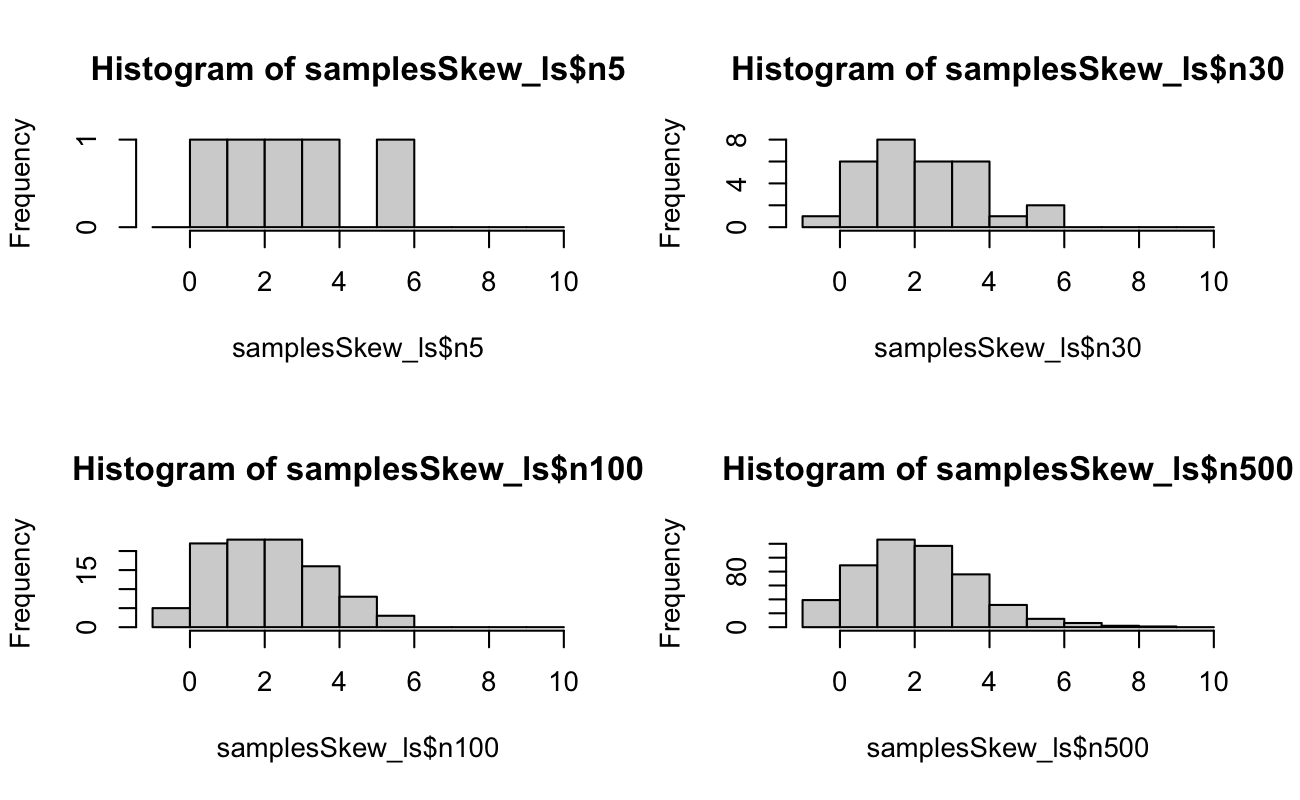
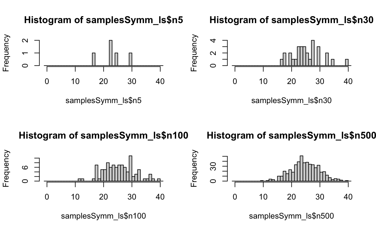
4.3 Example Random Samples
Code
set.seed(20150516)N <-5xSymm <-rpois(n =500, lambda =25)samplesSymm_ls <-list(n5 = xSymm[1:5],n30 = xSymm[1:30],n100 = xSymm[1:100],n500 = xSymm)binsSymm_int <-seq.int(from =-1, to =max(xSymm) +1, by =1)xSkew <-rpois(n =500, lambda =2.5)samplesSkew_ls <-list(n5 = xSkew[1:5],n30 = xSkew[1:30],n100 = xSkew[1:100],n500 = xSkew)binsSkew_int <-seq.int(from =-1, to =max(xSkew) +1, by =1)# we are drawing until we reach N successes, so the upper limit should be # N * (1 / min(prob)) + epsilonrm(xSymm, xSkew)
After the Herculean effort to derive this distribution, showing that it is a distribution is downright pedestrian in comparison.
4.4.1 The Distribution is Non-negative
As we already know, \(\lambda > 0\), \(t \ge 0\), and \(k \in 0 \cup\mathbb{N}\). Thus \((\lambda t)^k \ge 0\). Further, the exponential and factorial functions are non-negative. Thus, \(f_{\text{Poisson}}(k|\lambda t) \ge 0\).
4.4.2 The Total Probability is 1
Let’s recall the MacLaurin Series Expansion for the exponential function: \[
e^x \equiv \sum_{n = 0}^{\infty} \frac{x^n}{n!}.
\] This should give us a big hint for how were are going to integrate the Poisson distribution. Recall that the support for \(k\) is the set of 0 and all positive integers up to \(\infty\); that is \(\mathcal{S}(k) = [0,\infty) \in \mathbb{Z}\). Thus, we substitute the MacLaurin Series as follows: \[
\begin{aligned}
\int_{\mathcal{S}(k)} dF(k|\lambda t) &= \sum_{k = 0}^{\infty} \frac{(\lambda t)^k}{k!} e^{-\lambda t} \\
&= e^{-\lambda t} \sum_{k = 0}^{\infty} \frac{(\lambda t)^k}{k!} \\
&= e^{-\lambda t} \left[ e^{\lambda t} \right] \\
&= 1.
\end{aligned}
\]
4.5 Derive the Moment Generating Function
The MGF is found similarly, by (again) applying the MacLaurin Series expansion for \(e^x\). Note that we are using \(s\) as the nuisance parameter of the MGF instead of \(t\) because we already use \(\lambda t\) as the parameter of the Poisson Distribution Thus, \[
\begin{aligned}
M_k(s) &= \int_{\mathcal{S}(k)} e^{sk} dF(k|\lambda t) \\
&= \sum_{k = 0}^{\infty} e^{sk} \frac{(\lambda t)^k}{k!} e^{-\lambda t} \\
&= e^{-\lambda t} \sum_{k = 0}^{\infty} \frac{(e^s \lambda t)^k}{k!} \\
&= e^{-\lambda t} e^{e^s \lambda t} \\
&= \exp\left[ -\lambda t + e^s \lambda t \right] \\
&= \exp\left[ \lambda t (e^s - 1) \right].
\end{aligned}
\]
4.6 Method of Moments Estimates from Observed Data
Let’s generate some random data across 7 experiments. We assume that these 7 experiments represent 7 identical and fixed periods of time wherein to count events, with an average of with \(\lambda t = 5\) events in each interval:
If these data are the counts of patient visits to a clinic in these 7 time intervals, we can see that there were 7, 3, 5, 8, 4, 1, 4 patients in each interval. Now that we have the MGF and a sample of data, we can estimate the Poisson “rate” parameter \(\lambda t\).
4.6.1\(\mathbb{E}[k]\)
Recall that our MGF nuisance parameter is \(s\), not \(t\); \(\lambda t\) is the Poisson parameter. Now consider \[
\begin{aligned}
M_k(s) &= \exp[ \lambda t (e^s - 1) ] \\
\Longrightarrow \frac{d}{ds} M_k(s) &= \frac{d}{ds} \exp[ \lambda t (e^s - 1) ] \\
&= \exp[ \lambda t (e^s - 1) ] \frac{d}{ds} \lambda t (e^s - 1) \\
&= \exp[ \lambda t (e^s - 1) ] \lambda t e^s \\
&= \lambda t \exp[ \lambda t (e^s - 1) + s].
\end{aligned}
\] Thus, \[
\begin{aligned}
M_k^{\prime}(s) &= \lambda t \exp[ \lambda t (e^s - 1) + s] \\
\Longrightarrow M_k^{\prime}(0) &= \lambda t \exp[ \lambda t (e^{[0]} - 1) + [0]] \\
&= \lambda t \exp[ \lambda t (1 - 1) ] \\
&= \lambda t \exp[ 0 ] \\
&= \lambda t \\
&= \mathbb{E}[k].
\end{aligned}
\]
4.6.2\(\mathbb{E}[k^2]\) and \(\text{Var}[k]\)
Similarly, \[
\begin{aligned}
M_k^{\prime}(s) &= \lambda t \exp[ \lambda t (e^s - 1) + s] \\
\Longrightarrow M_k^{\prime\prime}(s) &= \frac{d}{ds} \lambda t \exp[ \lambda t (e^s - 1) + s] \\
&= \lambda t \exp[ \lambda t (e^s - 1) + s] \frac{d}{ds} [ \lambda t (e^s - 1) + s] \\
&= \lambda t [ \lambda t e^s + 1] \exp[ \lambda t (e^s - 1) + s].
\end{aligned}
\] Evaluating this second derivative at 0 yields \[
\begin{aligned}
M_k^{\prime\prime}(0) &= \lambda t [ \lambda t e^{[0]} + 1] \exp[ \lambda t (e^{[0]} - 1) + [0]] \\
&= \lambda t (\lambda t [1] + 1) \exp[\lambda t (1 - 1)] \\
&= \lambda t (\lambda t + 1) \\
&= \mathbb{E}[k^2].
\end{aligned}
\] Therefore, \[
\begin{aligned}
\text{Var}[k] &= \mathbb{E}[k^2] - \left[ \mathbb{E}[k] \right]^2 \\
&= \lambda t (\lambda t + 1) - [\lambda t]^2 \\
&= (\lambda t)^2 + \lambda t - (\lambda t)^2 \\
&= \lambda t.
\end{aligned}
\]
4.6.3 Solving the System
We now see the trivial solution to our problem: the Poisson distribution has the same estimates for mean and variance. Thus, \(\hat{\lambda}_{\text{MoM}} = \bar{k}\). For our example data, where the true value of \(\lambda t\) was 5, we see the Method of Moments estimate is
Code
mean(Poisk_int)[1] 4.57
4.7 Maximum Likelihood Estimators
For this last section, we will slightly change the parametrization of the Poisson Distribution. Let the Poisson rate be \(r = \lambda t\). Consider a sample \(\textbf{k}_i \overset{iid}{\sim} \text{Pois}(r),\ i = 1, 2, \ldots, n\). The log-likelihood is then \[
\begin{aligned}
f_{\text{Pois}}(k|r) &\equiv \frac{r^k}{k!}e^{-r} \\
\Longrightarrow \mathcal{L}(r|\textbf{k}) &= \prod_{i = 1}^n \frac{r^{k_i}}{k_i!}e^{-r} \\
\Longrightarrow \ell(r|\textbf{k}) &= \log \left[ \prod_{i = 1}^n \frac{r^{k_i}}{k_i!}e^{-r} \right] \\
&= \sum_{i = 1}^n \log \left[ \frac{r^{k_i}}{k_i!}e^{-r} \right] \\
&= \sum_{i = 1}^n \left[ k_i\log(r) - \log(k_i!) - r \right] \\
&= \log(r) \left[ \sum_{i = 1}^n k_i \right] - \left[ \sum_{i = 1}^n \log(k_i!) \right] - nr.
\end{aligned}
\]
Therefore, we find the extreme values of this log-likelihood by \[
\begin{aligned}
\ell(r|\textbf{k}) &= \log(r) \left[ \sum_{i = 1}^n k_i \right] - \left[ \sum_{i = 1}^n \log(k_i!) \right] - nr \\
\Longrightarrow \frac{\partial}{\partial r} \ell(r|\textbf{k}) &= \frac{\partial}{\partial r} \left( \log(r) \left[ \sum_{i = 1}^n k_i \right] - \left[ \sum_{i = 1}^n \log(k_i!) \right] - nr \right) \\
&= \frac{1}{r} \left[ \sum_{i = 1}^n k_i \right] - 0 - n \\
&= \frac{1}{r} [n\bar{k}] - n \\
\Longrightarrow 0 &\overset{\text{set}}{=} \frac{n\bar{k}}{\hat{r}} - n \\
\Longrightarrow n\hat{r} &= n\bar{k} \\
\Longrightarrow \hat{r} &= \bar{k}.
\end{aligned}
\] We have found that \(\hat{r} = \bar{k}\) yields an extreme value of \(\ell(r|\textbf{k})\), but we need to take the second derivative to confirm that it is a maximum. Then, \[
\begin{aligned}
\frac{\partial}{\partial r} \ell(r|\textbf{k}) &= \frac{1}{r} [n\bar{k}] - n \\
\Longrightarrow \frac{\partial^2}{\partial r^2} \ell(r|\textbf{k}) &= \frac{\partial}{\partial r} \left[\frac{1}{r} [n\bar{k}] - n \right] \\
&= -\frac{n\bar{k}}{r^2} \\
&< 0.
\end{aligned}
\] Ergo, \(\hat{r}_{\text{MLE}} = \bar{k}\).
 In the above picture (from the engineers at