Consider the outcomes of \(n\) independent and identical Bernoulli trials, \(k_i \overset{iid}{\sim} \text{Bern}(p),\ \forall i \in \{1, 2, \ldots, n\}\). We play a game where we “win” as soon as we flip enough heads. We pretend that we have a time machine, and we travel forward in time until right before the exact Bernoulli trial in which the “winning” coin flip happens. For example, imagine a game where, as soon as we’ve flipped 5 heads total, we win. We hop in our time machine and travel forward until we are just about to flip the 5th head. Let \(Y_n = \sum_i k_i\) be the (cumulative) count of successes so far in the game; for example, if we win at the \(5^{\text{th}}\) heads flipped, then we would have already seen four heads flipped this game. Let \(G_m\) be the flip number in which we will observe the \(m^{\text{th}}\) success (where \(m \ge 1\)). The probability of winning the game on coin flip \(m\) is then \[
\mathbb{P}[G_m = n] = \mathbb{P}[Y_{n - 1} = m - 1]\times\mathbb{P}[k_n = 1];
\] that is, the probability we win the game now, on flip \(n\), is the probability that we’ve seen \(m - 1\) heads in the last \(n - 1\) flips, times the probability that the very next flip (flip \(n\)) will be a heads. Recall that \(k_i \overset{iid}{\sim} \text{Bern}(p)\), so the probability that we saw \(m - 1\) successes in \(n - 1\) trials follows the Binomial distribution, where \[
\mathbb{P}[Y_{n - 1} = m - 1] = {n - 1 \choose m - 1} p^{m - 1} (1 - p)^{n - m}.
\] Since, by definition, \(\mathbb{P}[k_n = 1] = p\), then \[
\begin{aligned}
\mathbb{P}[G_m = n] &= {n - 1 \choose m - 1} p^{m - 1} (1 - p)^{n - m} \times p \\
&= {n - 1 \choose m - 1} p^{m} (1 - p)^{n - m},
\end{aligned}
\] which is a parametrization of the Negative Binomial Distribution.
While using counts of successes in total Bernoulli trials (\(m\) successes out of \(n\) trials) offers a clear derivation of this distribution, most of the time the Negative Binomial distribution is parametrized in terms counts of successes, \(r = m\), and failures, \(k = n - m\). Thus, \(n = k + r\) and \(m = r\). So, for \(k \in \{\mathbb{N} \cup 0\}\) and \(r \ge 1\), \[
\begin{aligned}
f_{\text{NB}}(m, n|p) &\equiv {n - 1 \choose m - 1} p^{m} (1 - p)^{n - m} \\
\Longrightarrow f_{\text{NB}}(r, k|p) &= {k + r - 1 \choose r - 1} p^{r} (1 - p)^{k} \\
&= \frac{(k + r - 1)!}{(r - 1)!([k + r - 1] - [r - 1])!} p^{r} (1 - p)^{k} \\
&= \frac{(k + r - 1)!}{(r - 1)!(k + r - 1 - r + 1)!} p^{r} (1 - p)^{k} \\
&= \frac{(k + r - 1)!}{k!(r - 1)!} p^{r} (1 - p)^{k} \\
&= \frac{(k + r - 1)!}{k!([k + r - 1] - k)!} p^{r} (1 - p)^{k} \\
&= {k + r - 1 \choose k} p^{r} (1 - p)^{k},
\end{aligned}
\] which is the more common form of the Negative Binomial distribution.
3.2 Example Random Samples
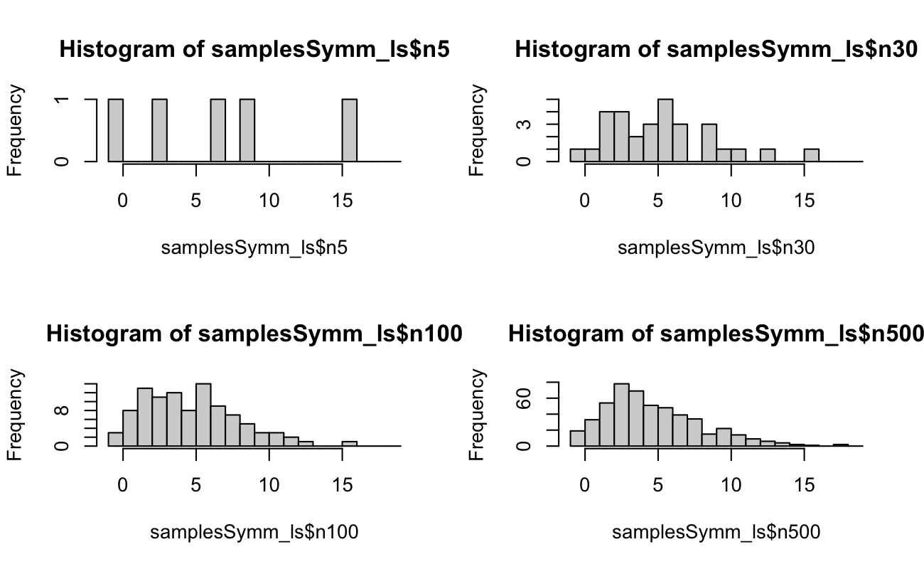
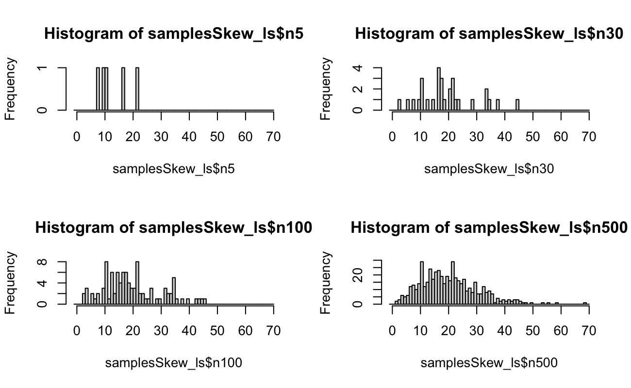
Code
set.seed(20150516)N <-5xSymm <-rnbinom(n =500, size = N, prob =0.5)samplesSymm_ls <-list(n5 = xSymm[1:5],n30 = xSymm[1:30],n100 = xSymm[1:100],n500 = xSymm)binsSymm_int <-seq.int(from =-1, to =max(xSymm) +1, by =1)xSkew <-rnbinom(n =500, size = N, prob =0.2)samplesSkew_ls <-list(n5 = xSkew[1:5],n30 = xSkew[1:30],n100 = xSkew[1:100],n500 = xSkew)binsSkew_int <-seq.int(from =-1, to =max(xSkew) +1, by =1)# we are drawing until we reach N successes, so the upper limit should be # N * (1 / min(prob)) + epsilonrm(xSymm, xSkew)
A Taylor (MacLaurin) Series expansion is a polynomial approximation of an \(n\)-differentiable real-valued function \(f\) around a point \(a\) (the MacLaurin Series is a special case when \(a = 0\)). Let \(f^{(n)}(a)\) denote the \(n^{\text{th}}\) derivative of the function \(f\) evaluated at \(a\). Then the \(n^{\text{th}}\)-order Taylor Series approximation of \(f\) in a neighbourhood of \(a\) is given by \[
f(x) \approx f(a) + \frac{f^{\prime}(a)}{1!}(x - a)^1 + \frac{f^{\prime\prime}(a)}{2!}(x - a)^2 + \ldots + \frac{f^{(n)}(a)}{n!}(x - a)^n.
\] If \(f\) is infinitely-differentiable, then this series can be continued in perpetuity, and the approximation becomes exact. That is \[
f(x) = \sum_{n = 0}^{\infty} \frac{f^{(n)}(a)}{n!}(x - a)^n.
\]
3.3.2 Infinite Geometric Series
For a real number \(|r| < 1\), the Geometric Series is the infinite-term MacLaurin Series form for the ratio below: \[
\frac{b}{1 - r} = \sum_{k = 0}^{\infty} br^k.
\]Proof: We presented the definition of the Taylor Series for an infinitely-differentiable function \(f\) above. We need the functional form of the \(n^{\text{th}}\) derivative of \((1 - r)^{-1}\) evaluated at an arbitrary point \(a\), where \(|r| < 1\). These derivatives are given as \[
\begin{align}
f^{(0)}(a) &= (1 - a)^{-1} \\
f^{(1)}(a) &= (-1)(1 - a)^{-2}(-1) =& (1 - a)^{-2}\\
f^{(2)}(a) &= (-2)(1 - a)^{-3}(-1) =& 2(1 - a)^{-3}\\
f^{(3)}(a) &= (-3)(2)(1 - a)^{-4}(-1) =& 3\times2(1 - a)^{-4}\\
f^{(4)}(a) &= (-4)(3)(2)(1 - a)^{-5}(-1) =& 4!(1 - a)^{-5}\\
\vdots \\
f^{(n)}(a) &= n!(1 - a)^{-(n + 1)}.
\end{align}
\] We evaluate these derivatives at \(a = 0\), yielding \(f^{(n)}(0) = n!(1 - 0)^{-(n + 1)} = n!\). Therefore, evaluating the MacLaurin Series for this ratio (the Taylor Series at \(a = 0\)) yields \[
\begin{align}
f(r) = \frac{1}{1 - r} &= \sum_{n = 0}^{\infty} \frac{f^{(n)}(0)}{n!}(r - 0)^n \\
&= \sum_{n = 0}^{\infty} \frac{\left[ n! \right]}{n!} r^n \\
&= \sum_{n = 0}^{\infty} r^n.
\end{align}
\] Hence, after changing the index of summation from \(n\) to \(k\) and multiplying both sides by \(b\), we have \[
\frac{b}{1 - r} = \sum_{k = 0}^{\infty} br^k.
\]
3.3.3 Newton’s Binomial Theorem
Newton’s Binomial Theorem allows us to generalize the Infinite Geometric Series for \(|r| < 1\) from exponents other than \(-1\) as follows1: \[
b(1 + r)^{\alpha} = \sum_{n = 0}^{\infty} {\alpha \choose n} br^n.
\]Proof: We will follow the same MacLaurin Series derivation for \((1 + r)^{\alpha}\) here as well, where the only major difference is that we have \(+r\) instead of \(-r\). The \(n\) derivatives evaluated at \(r = r_0\) are then \[
\begin{align}
f^{(0)}(r_0) &= (1 + r_0)^{\alpha} \\
f^{(1)}(r_0) &= (\alpha)(1 + r_0)^{\alpha - 1} \\
f^{(2)}(r_0) &= (\alpha)(\alpha - 1)(1 + r_0)^{\alpha - 2} \\
f^{(3)}(r_0) &= (\alpha)(\alpha - 1)(\alpha - 2)(1 + r_0)^{\alpha - 3} \\
\vdots \\
f^{(n)}(r_0) &= \left[ (\alpha)(\alpha - 1)(\alpha - 2) \ldots (\alpha - n + 1) \right] (1 + r_0)^{\alpha - n} \\
&= \left[ (\alpha)(\alpha - 1)(\alpha - 2) \ldots (\alpha - n + 1) \right] \frac{(\alpha - n)!}{(\alpha - n)!} (1 + r_0)^{\alpha - n} \\
&= \frac{\alpha!}{(\alpha - n)!} (1 + r_0)^{\alpha - n} \\
\Longrightarrow f^{(n)}(0) &= \frac{\alpha!}{(\alpha - n)!} (1 + 0)^{\alpha - n} \\
&= \frac{\alpha!}{(\alpha - n)!}.
\end{align}
\] Therefore, \[
\begin{aligned}
b(1 + r)^{\alpha} &= b \sum_{n = 0}^{\infty} \frac{f^{(n)}(0)}{n!} (r - 0)^n \\
&= b \sum_{n = 0}^{\infty} \frac{\left[ \frac{\alpha!}{(\alpha - n)!} \right]}{n!} r^n \\
&= b \sum_{n = 0}^{\infty} \frac{\alpha!}{n!(\alpha - n)!} r^n \\
&= \sum_{n = 0}^{\infty} {\alpha \choose n} br^n
\end{aligned}
\]
3.3.4 The Gamma Function
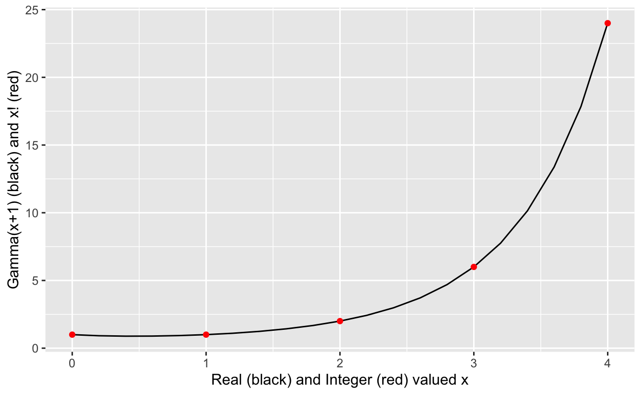
As a preliminary comment, we could spend literal weeks discussing and proving the many properties of a function called the Gamma Function, and we will discuss it in much greater depth as we progress further into these lessons on various statistical distributions. However, for now, suffice it to say that the Gamma Function is a generalization of the factorial function. Visually, it “connects the dots” between the integer factorial values. To see this, we will generate factorial and Gamma values from 0 to 4.
Code
factorialValues_df <-data.frame(n =0:4,nFact =factorial(0:4))gammaValues_df <-data.frame(x =seq(from =0, to =4, length.out =21),xGamma =gamma(seq(from =0, to =4, length.out =21) +1))
Now let’s visualize these two sets of values.
Code
library(ggplot2)ggplot() +geom_line(data = gammaValues_df, aes(x = x, y = xGamma)) +geom_point(data = factorialValues_df, aes(x = n, y = nFact), color ="red") +labs(x ="Real (black) and Integer (red) valued x",y ="Gamma(x+1) (black) and x! (red)" )
So, we see that the Gamma Function is one (of potentially many) smooth interpolations between the values of \(x!\) evaluated at each non-negative integer. However, it can be extended to the negative (non-integer) numbers and even the complex plane. At its most complex (for this class anyway), the Weierstrass’s Definition of the Gamma Function for all complex values of \(z = a + bi\) except for the negative integers is \[
\Gamma(z) \equiv \frac{e^{-\gamma z}}{z} \prod_{n = 1}^{\infty} \left( 1 + \frac{z}{n} \right)^{-1} e^{\frac{z}{n}},
\] where \(\gamma \approx 0.577\) is the Euler-Mascheroni constant.
Thankfully, we don’t have to use this version, we only have to know that it exists. The version that we will use most is the representation of the Gamma Function when the Real component \(z\) is positive; that is, when \(a > 0\). We represent this condition symbolically as \(\mathbb{R}(z) > 0\). It’s also worth noting that this includes all the positive real numbers as well, because \(b\) in \(z = a + bi\) could be \(0\). So, the “common form” of the Gamma Function is \[
\Gamma(z) = \int_0^{\infty} t^{z - 1}e^{-t}dt,\ \mathbb{R}(z) > 0.
\] Finally, in the simplest case, if \(z\) can be written as a non-negative integer \(n\), then we get the simplest form of all: \[
\Gamma(n) \equiv (n - 1)!.
\] For the next few lessons (at least until we get to the Gamma and Beta Distributions), we won’t yet need to formalize or prove any properties of this function. For now, we simply need to know that it’s possible to extend the factorial beyond the integers.
3.3.5 “Negative” Binomial Coefficients
This is a specific form of the Generalized Binomial Coefficient that allows us to extend the mathematical relationship of the binomial theorem beyond its usual applications of combinations (where \(n\) and \(k\) are required to be non-negative integers). This generalization yields the following property, which we will shortly prove: \[
{-a \choose b} \equiv (-1)^b {a + b - 1 \choose b}.
\]
Proof: Consider \(a,b \in \mathbb{R}\) and further recall by the above definition of the Gamma Function that the factorial operator can be extended beyond the integers. Even though we do not define how to calculate such a value, we will only need to know for this proof that such numbers could possibly exist. Thus, \[
\begin{aligned}
{-a \choose b} &= \frac{(-a)!}{b!(-a - b)!} \\
&= \frac{(-a)(-a - 1)(-a - 2)\ldots(-a - b + 1)(-a - b)!}{b!(-a - b)!} \\
&= \frac{(-a)(-a - 1)(-a - 2)\ldots(-a - b + 1)}{b!} \\
&= (-1)^b\frac{(a)(a + 1)(a + 2)\ldots(a + b - 1)}{b!} \\
&= (-1)^b\frac{(a + b - 1)\ldots(a + 2)(a + 1)(a)}{b!} \times \frac{(a - 1)!}{(a - 1)!} \\
&= (-1)^b\frac{(a + b - 1)!}{b!(a - 1)!} \\
&= (-1)^b\frac{(a + b - 1)!}{b!([a + b - 1] - b)!} \\
&= (-1)^b {a + b - 1 \choose b}.
\end{aligned}
\]
3.4 Show that this is a Distribution
We first consider the parametrization with \(m\) successes out of \(n\) trials. That is, \[
f_{\text{NB}}(n|m,p) \equiv {n - 1 \choose m - 1} p^{m} (1 - p)^{n - m}, 1 \le m \le n < \infty,\ p\in (0,1).
\] Note that \(m \ge 1\) because we are counting the number of trials until we see at least one success. Also note that \(n\) has no upper bound. If the “game” is the United States Men’s Soccer team winning the FIFA World Cup, the number of World Cups necessary, \(n\), for this event, \(m = 1\), to occur \(\to\infty\).
3.4.1 The Distribution is Non-negative
As we already know, \(p\in (0,1)\). Thus \(p^m,\ (1 - p)^{n - m} > 0\). Further, \(1 \le m \le n < \infty\), so Binomial Coefficient will never be smaller than 1. Thus, for \(p\in (0,1)\), \(f_{\text{NB}}(m, n|p) > 0\), and for \(p\) outside this defined range of probability, \(f_{\text{NB}}(m, n|p) \equiv 0\) by definition. Thus, \(f_{\text{NB}}(m, n|p) \ge 0\ \forall p\).
3.4.2 The Total Probability is 1
This proof is considerably more involved than the proof for the Binomial Distribution; I follow this guide from Mathematics Stack Exchange. We will use proof by induction, infinite geometric series, and Pascal’s Rule of factorials. These topics are covered in the “Formal Foundations” subsections of this lesson and the previous lesson on the Binomial Distribution. Let’s begin by defining a shorthand form of the Riemman-Stieljes integral of the Negative Binomial Distribution over the support of \(n\); let \[
S_m \equiv \int\limits_{\mathcal{S}(n|m)} dF(n|m,p) = \sum_{n = m}^{\infty} {n - 1 \choose m - 1} p^m (1 - p)^{n - m},\ \forall m\in\mathbb{N}.
\]
The base case is the event when \(m = 1\). So we must show that \(S_1 = 1\). First, recall that there is only 1 way to “choose” 0 events, so \[
\begin{aligned}
S_1 &= \sum_{n = 1}^{\infty} {n - 1 \choose 1 - 1} p^1 (1 - p)^{n - 1} \\
&= p \sum_{n = 1}^{\infty} {n - 1 \choose 0} (1 - p)^{n - 1} \\
&= p \sum_{n = 1}^{\infty} (1) (1 - p)^{n - 1} \\
&= p \sum_{k + 1 = 1}^{\infty} (1 - p)^k,\ \text{for}\ n = k + 1 \\
&= p \sum_{k = 0}^{\infty} (1 - p)^k \\
&\qquad \text{\emph{Infinite Geometric Series...}} \\
&= p \left[ \frac{1}{1 - [1 - p]} \right],\ |1 - p| < 1 \\
&= \frac{p}{1 - 1 + p} \\
&= 1.
\end{aligned}
\] The hypothesis is then that \(S_m = 1\). That is, we assume that \[
S_m = \sum_{n = m}^{\infty} {n - 1 \choose m - 1} p^m (1 - p)^{n - m} = 1.
\] Our induction will be to assume the hypothesis is true for \(m\) and show that this implies that it is also true for \(m+1\).
Now, using this \(S_m\) notation, and recalling Pascal’s Rule: \[
\begin{aligned}
S_{m + 1} &= \sum_{n = m + 1}^{\infty} {n - 1 \choose m + 1 - 1} p^{m + 1} (1 - p)^{n - (m + 1)} \\
&= \sum_{n = m + 1}^{\infty} {n - 1 \choose m} p^{m + 1} (1 - p)^{n - m - 1} \\
&\qquad \text{\emph{Pascal's Rule...}} \\
&= \sum_{n = m + 1}^{\infty} \left[ {n - 2 \choose m} + {n - 2 \choose m - 1} \right] p^{m + 1} (1 - p)^{n - m - 1} \\
&= \sum_{n = m + 1}^{\infty} {n - 2 \choose m} p^{m + 1} (1 - p)^{n - m - 1} + \sum_{n = m + 1}^{\infty} {n - 2 \choose m - 1} p^{m + 1} (1 - p)^{n - m - 1}.
\end{aligned}
\] At this point, we’d like to pull out something that looks like \(S_m\), because we are assuming that equals 1. Let’s change the summation index by letting \(j = n - 1 \Rightarrow n = j + 1\) and pick back up: \[
\begin{aligned}
S_{m + 1} &= \sum_{[j + 1] = m + 1}^{\infty} {[j + 1] - 2 \choose m} p^{m + 1} (1 - p)^{[j + 1] - m - 1} + \sum_{[j + 1] = m + 1}^{\infty} {[j + 1] - 2 \choose m - 1} p^{m + 1} (1 - p)^{[j + 1] - m - 1} \\
&= \sum_{j = m}^{\infty} {j - 1 \choose m} p^{m + 1} (1 - p)^{j - m} + \sum_{j = m}^{\infty} {j - 1 \choose m - 1} p^{m + 1} (1 - p)^{j - m} \\
&= (1 - p) \sum_{j = m}^{\infty} {j - 1 \choose m} p^{m + 1} (1 - p)^{j - m - 1} + p \sum_{j = m}^{\infty} {j - 1 \choose m - 1} p^{m} (1 - p)^{j - m} \\
&= (1 - p) \sum_{j = m}^{\infty} {j - 1 \choose m} p^{m + 1} (1 - p)^{j - m - 1} + pS_m \\
&= (1 - p) \left[ {m - 1 \choose m} p^{m + 1} (1 - p)^{m - m - 1} + \sum_{j = m + 1}^{\infty} {j - 1 \choose m} p^{m + 1} (1 - p)^{j - m - 1} \right] + pS_m \\
&= (1 - p) \left[ 0 + \sum_{j = m + 1}^{\infty} {j - 1 \choose m} p^{m + 1} (1 - p)^{j - m - 1} \right] + pS_m.
\end{aligned}
\] The last line requires us to observe that \({m - 1 \choose m} = 0\ \forall m \in \mathbb{N}\) because there are 0 ways to choose \(m\) objects from a set of \(m - 1\) objects. For our final component of the induction step, we notice that the second term in the brackets is \(S_{m+1}\) using an index of \(j\) instead of \(n\). Thus, \[
\begin{aligned}
S_{m + 1} &= (1 - p) \left[\sum_{j = m + 1}^{\infty} {j - 1 \choose m} p^{m + 1} (1 - p)^{j - m - 1} \right] + pS_m \\
&= (1 - p) \left[ S_{m + 1} \right] + pS_m \\
&= S_{m + 1} - pS_{m + 1} + pS_m \\
\Longrightarrow 0 &= pS_m - pS_{m + 1} \\
\Longrightarrow S_{m + 1} &= S_m.
\end{aligned}
\] Because we assumed that \(S_m = 1\) at our hypothesis step, we then have that \(S_m = 1 \Rightarrow S_{m + 1} = 1\), which completes our proof. Thus, \(\forall m \in \mathbb{N}\), \[
\sum_{n = m}^{\infty} {n - 1 \choose m - 1} p^m (1 - p)^{n - m} = 1.
\]
3.5 Derive the Moment Generating Function
In my opinion, it’s easier to derive the MGF of the Negative Binomial when we use the \(k,r\) parametrization (where \(r \ge 1\) is the number of successes and \(k \ge 0\) is the number of failures). Thus, \[
\begin{aligned}
f_{\text{NB}}(k,r|p) &= {k + r - 1 \choose k} p^r (1 - p)^k \\
\Longrightarrow M_k(t) &= \int_{\mathcal{S}(k)} e^{tk} dF(k,r|p) \\
&= \sum_{k = 0}^{\infty} e^{tk} {k + r - 1 \choose k} p^r (1 - p)^k \\
&= p^r \sum_{k = 0}^{\infty} {k + r - 1 \choose k} \left[ e^{t}(1 - p) \right]^k \\
&\qquad \text{\emph{Generalized/Negative Binomial Coefficient...}} \\
&= p^r \sum_{k = 0}^{\infty} \left[ (-1)^k {-r \choose k} \right] \left[ e^{t}(1 - p) \right]^k \\
&= p^r \sum_{k = 0}^{\infty} {-r \choose k} \left[ -e^{t}(1 - p) \right]^k \\&\qquad \text{\emph{Newton's Binomial Theorem...}} \\
&= p^r \left( 1 + \left[ -e^{t}(1 - p) \right] \right)^{[-r]}.
\end{aligned}
\] To correctly invoke Newton’s Binomial Theorem in this last step, we must recall that Moment Generating Functions are defined within an \(\epsilon\)-neighbourhood of 0. Therefore, \(e^t(1 - p) \approx (1)(1 - p)\), which we can safely bound between \(0\) and \(1\) for arbitrarily small \(\epsilon\), just as long as \(p \ne \{0, 1\}\) (as in, as long as neither failure nor success are guaranteed). Thus, \[
M_k(t) = \left[ \frac{p}{1 - e^{t}(1 - p)} \right]^r.
\]
3.6 Method of Moments Estimates from Observed Data
If we see \(n\) repeated Negative Binomial experiments, then we must already know the following information:
We know that in each of the \(n\) experiments, by definition we observed \(r\) successes.
We know that in each experiment, the “games” or “trials” were conducted independently until all \(r\) successes were observed. Thus, the number of games in each experiment vary, and the probability of winning in each game, \(p\), does not change (but it is unknown in real life).
Based on the first two facts, we then know that the “data” in repeated Negative Binomial experiments is the count of failures observed in each experiment until all \(r\) successes were observed. We denote these counts as \(k_i,\ i = 1, 2, \ldots n\).
Therefore, our observed data is \(\textbf{k} = \langle k_1, k_2,\ldots,k_n\rangle\), the counts of the number of failures in each experiment until success number \(r\) was observed. Let’s generate some random data with \(r = 5\) and \(p = 0.35\) across 7 experiments:
As we can see, in order to achieve 5 wins total in each experiment, we needed 5 + 13, 10, 3, 7, 18, 9, 12 “games” in those experiments. Now that we have the MGF and a sample of data, we can:
Find \(\mathbb{E}[k]\), \(\mathbb{E}[k^2]\), and \(\text{Var}[k]\), then
Create (and solve) a system of two equations by setting \(\mathbb{E}[k] = \bar{k}\) and \(\text{Var}[k] = s^2\).
We now have the following non-linear system of equations to solve: \[
\begin{aligned}
\mathbb{E}[k] &: \frac{r(1 - p)}{p} = \bar{k} \\
\text{Var}[k] &: \frac{r(1 - p)}{p^2} = s^2
\end{aligned}
\] We will first isolate \(r\) as a function of \(s^2\). In most real data scenarios, we know \(r\), but for completion we will here assume it’s unknown. Thus, \[
\begin{aligned}
s^2 &= \frac{r(1 - p)}{p^2} \\
\Longrightarrow r &= \frac{p^2s^2}{1 - p} \\
\Longrightarrow \bar{k} &= \left[ \frac{p^2s^2}{1 - p} \right] \times \frac{(1 - p)}{p} \\
&= ps^2 \\
\Longrightarrow \hat{p}_{MoM} = \frac{\bar{k}}{s^2}.
\end{aligned}
\] Subsequently, if we had to estimate \(r\) (which is unlikely), then \[
\begin{aligned}
\bar{k} &= \frac{r(1 - p)}{p} \\
&= \frac{r\left( 1 - \left[ \frac{\bar{k}}{s^2} \right] \right)}{\left[ \frac{\bar{k}}{s^2} \right]} \\
&= r\frac{s^2}{\bar{k}} \left[ 1 - \frac{\bar{k}}{s^2} \right] \\
\Longrightarrow \bar{k} &= r \left[ \frac{s^2}{\bar{k}} - 1 \right] \\
\Longrightarrow \bar{k}^2 &= r (s^2 - \bar{k}) \\
\Longrightarrow \hat{r}_{MoM} &= \frac{\bar{k}^2}{s^2 - \bar{k}}.
\end{aligned}
\] For this data, we know that \(r\) = 5, and we generated data for \(n\) = 7 trials with \(p\) equal to 0.35. Thus, given the observed data, we estimate \(\hat{p}_{MoM}\) as
Code
mean(NBk_int) /var(NBk_int)[1] 0.456
3.7 Maximum Likelihood Estimators
Because we should know \(r\) in advance of the experiment, and because \(\textbf{k}\) is the observed counts across \(n\) experiments, the only unknown is \(p\). The likelihood function is then \[
\mathcal{L}(p|\textbf{k},r) = \prod\limits_{i = 1}^n {k_i + r - 1 \choose k_i} p^r (1 - p)^k_i,\ p\in (0,1).
\] We then find the extreme value of \(\mathcal{L}\) by \[
\begin{aligned}
\ell(p|\textbf{k},r) &= \sum\limits_{i = 1}^n \log\left[ {k_i + r - 1 \choose k_i} p^r (1 - p)^{k_i} \right] \\
&= \sum\limits_{i = 1}^n \left[ \log{k_i + r - 1 \choose k_i} + r\log(p) + k_i \log(1 - p) \right] \\
&= nr\log(p) + \log(1 - p) \sum\limits_{i = 1}^n k_i + \sum\limits_{i = 1}^n \log{k_i + r - 1 \choose k_i} \\
&= nr\log(p) + n\bar{k}\log(1 - p) + \sum\limits_{i = 1}^n \log{k_i + r - 1 \choose k_i} \\
\Longrightarrow \frac{\partial\ell(p|\textbf{k},r)}{\partial p} &= \frac{nr}{p} - \frac{n\bar{k}}{1 - p} + 0 \\
\Longrightarrow 0 &\overset{\text{set}}{=} \frac{nr}{\hat{p}} - \frac{n\bar{k}}{1 - \hat{p}} \\
\Longrightarrow 0 &= nr(1 - \hat{p}) - n\bar{k}\hat{p} \\
&= nr - nr\hat{p} - n\bar{k}\hat{p} \\
\Longrightarrow nr &= \hat{p}(nr + n\bar{k}) \\
\Longrightarrow \hat{p} &= \frac{nr}{nr + n\bar{k}} \\
&= \frac{r}{r + \bar{k}}.
\end{aligned}
\] Now we need to confirm that this is indeed a maximum value, so we check the second derivative of the log-likelihood: \[
\begin{aligned}
\frac{\partial\ell(p|\textbf{k},r)}{\partial p} &= \frac{nr}{p} - \frac{n\bar{k}}{1 - p} \\
&= nrp^{-1} - n\bar{k}(1 - p)^{-1} \\
\Longrightarrow \frac{\partial^2\ell(p|\textbf{k},r)}{\partial p^2} &= -nrp^{-2} - (-1)n\bar{k}(1 - p)^{-2}(-1) \\
&= -\frac{nr}{p^2} - \frac{n\bar{k}}{(1 - p)^2} \\
&< 0,
\end{aligned}
\] as long as \(\{n,r\} >0\) and \(p\in(0,1)\). Thus, \(\hat{p}_{MLE} = \frac{r}{r + \bar{k}}\). For our observed data, with \(r\) = 5, this is
Code
r_int / (r_int +mean(NBk_int))[1] 0.327
Unlike in the Binomial Distribution case, where the two estimators were quite close, this ML estimate for \(p\) is much closer to the true value of \(p\) = 0.35 than the MoM estimate.
3.8 Exercises
3.8.1 The Geometric Distribution
When \(1 = m \le n\) (we are repeating trials until we observe the first success), the Negative Binomial Distribution reduces to the Geometric Distribution.
Derive this distribution
Find \(\mathbb{E}[n]\) and \(\text{Var}[n]\).
Find the MGF of this distribution.
Other exercises to be determined.
3.9 Footnotes
for the implications of “choosing” from values that aren’t necessarily integers, see the next subsection on the Gamma Function↩︎