When we derived the Exponential Distribution, we started with a Poisson process with rate \(\lambda\) and time interval length \(t\), and we asked “how long will we have to wait until we see the first patient?” The Erlang Distribution1 extends this to the total waiting time until patient number \(\alpha\in\mathbb{N}\) arrives, and the Gamma Distribution2 generalizes this to any \(\alpha\in\mathbb{R}^+\), removing the restriction that \(\alpha\) need be an integer. For this lesson, I’m following Clay Ford’s process3 to derive these distributions, but I’m deviating a bit where I think I can add some clarity. We will derive the Erlang Distribution first (because it follows a similar process to deriving the Exponential Distribution), then we will extend our derivation to the Gamma Distribution.
7.2 Formal Foundations
7.2.1 Leibniz’ Integral Rule
Let \(F(x)\) be a differentiable function over an interval \(x\in[a,b] \subset \mathbb{R}\) and let \(f(x)\) denote this derivative of \(F\). We know the First and Second Fundamental Theorems of Calculus4 state that \[
\begin{aligned}
(1)\qquad &\frac{d}{dx} \int f(x)dx = \frac{d}{dx} F(x) = f(x) \\
(2)\qquad &\int_a^b f(x)dx = F(b) - F(a).
\end{aligned}
\]Leibniz’ Integral Rule5 extends these theorems to allow more flexible bounds of integration and combines these results with the Chain Rule. Let \(a(x)\) and \(b(x)\) be finite-valued, differentiable functions. Then, for a differentiable function \(F(t)\) with derivative \(f(t)\), \[
\frac{d}{dx} \left[ \int_{a(x)}^{b(x)} f(t)dt \right] = f(b(x))\frac{d}{dx}b(x) - f(a(x))\frac{d}{dx}a(x).
\]
Proof: We assume that \(F\), \(f\), \(a\), and \(b\) are all nice functions that have the properties described above. Then, this result is shown by a straightforward application of the First and Second Fundamental Theorems and then the Chain Rule: \[
\begin{aligned}
\frac{d}{dx} \left[ \int_{a(x)}^{b(x)} f(t)dt \right] &= \frac{d}{dx} \Biggl [ F(b(x)) - F(a(x)) \Biggr ] \\
&= f(b(x))\frac{d}{dx}b(x) - f(a(x))\frac{d}{dx}a(x),
\end{aligned}
\] which completes our proof.
7.2.2 Integrating like a Statistician
To be honest, this “formal foundations” subsection is my favourite of all that I’ve included in this book. The idea is really simple: when you are integrating/summing a function over a fixed boundary (a definite integral6) or over a region that extends towards infinity (an improper unbounded integral7), then be on the lookout for the kernel8 of a statistical distribution. Because you know that distributions must integrate/sum to 1 over their entire support, you can often cancel out very complicated integral pieces if you can use algebra to turn them into the kernel of a distribution.
Let’s have an example. Consider this integral: \[
\int_{-\infty}^0 e^{3x-2}dx.
\] We could integrate this with the traditional \(u\)-substitution and improper limits procedures, or we could “look for the hidden distribution”. First, we want to flip the bounds of integration, replacing all \(x\) with \(-x\), so \[
\int_{-\infty}^0 e^{3x-2}dx = \int_0^{\infty} e^{3[-x]-2}dx = \int_0^{\infty} e^{-3x-2}dx.
\] Now this integral has the same support (\(\mathbb{R}^+\)) as quite a few statistical distributions, including the Weibull, Gamma, Rayleigh, Exponential, and \(\chi^2\) distributions. The integrand \(e^{-3x-2}\) looks similar to the probability function of the Exponential Distribution, so let’s try to use algebra to turn it into something that looks like \(\lambda e^{-\lambda t}\). We need to get rid of the \(-2\) in the exponent first: \[
\int_0^{\infty} e^{-3x-2}dx = \int_0^{\infty} e^{-3x}e^{-2}dx = \frac{1}{e^2} \int_0^{\infty} e^{-3x}dx.
\] This looks like the kernel of an Exponential Distribution with parameter \(\lambda = 3\). That’s good news, so \[
\frac{1}{e^2} \int_0^{\infty} e^{-3x}dx = \frac{3}{3e^2} \int_0^{\infty} e^{-3x}dx = \frac{1}{3e^2} \int_0^{\infty} 3e^{-3x}dx.
\] Finally, we remember that the integral of a probability function over its entire support is equal to 1, so \[
\frac{1}{3e^2} \int_0^{\infty} 3e^{-3x}dx = \frac{1}{3e^2} (1) = \frac{1}{3e^2}.
\] Therefore, \[
\int_{-\infty}^0 e^{3x-2}dx = \frac{1}{3e^2}.
\]
Now, for this example, you might say “that seemed like a really complex way to solve a simple problem.” And you’d be right. However, many integrals we encounter are far more challenging than this one, and learning to be on the lookout for kernels to appear in integrals is a prudent thing to do. For more examples, see this online homework page.9
7.3 Deriving the Distribution: The Erlang Distribution
As we mentioned above, we have a Poisson process with rate \(\lambda\) and time interval length \(t\), such as the number of patients visiting a clinic each hour. Now, assume that we have already observed \(\alpha - 1\) independent events (visits in this case). What would be the waiting time between event \(\alpha - 1\) and event \(\alpha\)? Let \(T\) be the time that event number \(\alpha\) takes place, and let \(t\) be the random variable. Then, because we’ve already observed \(\alpha - 1\) events so far, the probability that we observe \(\alpha\) total events before time \(t\) is the compliment to the probability that we observe event number \(\alpha\) after time \(t\), which is the same as 1 minus the probability that we observed all \(\alpha - 1\) events before time \(t\) in this Poisson process.
I know that’s a lot, but let’s walk through these statements symbolically: \[
\begin{aligned}
F(t) &= \mathbb{P}[T \le t] \\
&= 1 - \mathbb{P}[T > t] &(1)\ \\
&= 1 - F_{\text{Pois}}(k = \alpha - 1|\lambda, t) &(2),
\end{aligned}
\] where \(F_{\text{Pois}}\) is the cumulative probability function of the Poisson Distribution with rate \(\lambda\) and time interval \(t\). We move from equation (1) to (2) because the probability that the time of event number \(\alpha\) (that is, \(T\)) happens later (after \(t\)), is the same as the probability that all but one of the events have already happened (the count of events \(k\) so far, up to and including \(t\), equals \(\alpha - 1\)).
Then, as long as we can write down what \(F_{\text{Pois}}\) is, we get the Gamma (technically Erlang) Distribution, right? Easy enough… \[
\begin{aligned}
F(t|\alpha, \lambda) &= 1 - F_{\text{Pois}}(k = \alpha - 1|\lambda, t) \\
&= 1 - \int_{\mathcal{S}(k)} dF_{\text{Pois}}(k = \alpha - 1|\lambda, t) \\
&= 1 - \sum_{k = 0}^{\alpha - 1} \frac{(\lambda t)^k}{k!} e^{-\lambda t} \\
\Longrightarrow f(t|\alpha, \lambda) &= \frac{\partial}{\partial t} \left[ 1 - \sum_{k = 0}^{\alpha - 1} \frac{(\lambda t)^k}{k!} e^{-\lambda t} \right] \\
&= -\frac{\partial}{\partial t} \sum_{k = 0}^{\alpha - 1} \frac{(\lambda t)^k}{k!} e^{-\lambda t},
\end{aligned}
\] which looks exactly like the Gamma Distribution we know and love! Just kidding, this looks awful.
We have the probability function as the derivative of a summation, but we don’t have it in a form that’s easy to use or recognise. Recalling that both differentiation and summation are linear operators10, we can then swap the order of the two as needed. Let’s begin by first using the Product Rule, and then rearrange the difference of summations so that they almost entirely cancel: \[
\begin{aligned}
f(t|\alpha,\lambda) &= -\frac{\partial}{\partial t} e^{-\lambda t} \sum_{k = 0}^{\alpha - 1} \frac{(\lambda t)^k}{k!} \\
&\qquad \text{\emph{Product Rule}}\ \ldots \\
&= -\left\{ \left[ \frac{\partial}{\partial t} e^{-\lambda t} \right] \left[ \sum_{k = 0}^{\alpha - 1} \frac{(\lambda t)^k}{k!} \right] + e^{-\lambda t} \frac{\partial}{\partial t} \left[ \sum_{k = 0}^{\alpha - 1} \frac{(\lambda t)^k}{k!} \right] \right\}\\
&= -\left\{ \left[ -\lambda e^{-\lambda t} \right] \left[ \sum_{k = 0}^{\alpha - 1} \frac{(\lambda t)^k}{k!} \right] + e^{-\lambda t} \frac{\partial}{\partial t} \left[ \frac{(\lambda t)^0}{0!} + \sum_{k = 1}^{\alpha - 1} \frac{(\lambda t)^k}{k!} \right] \right\}\\
&= e^{-\lambda t} \left\{\left[ \sum_{k = 0}^{\alpha - 1} \frac{\lambda^{k+1} t^k}{k!} \right] - \frac{\partial}{\partial t} \left[ 1 + \sum_{k = 1}^{\alpha - 1} \frac{\lambda^k}{k!}t^k \right] \right\}\\
&\qquad \text{\emph{Differentiation is linear}}\ \ldots \\
&= e^{-\lambda t} \left\{ \left[ \frac{\lambda^{\alpha} t^{\alpha - 1}}{(\alpha - 1)!} + \sum_{k = 0}^{\alpha - 2} \frac{\lambda^{k+1} t^k}{k!} \right] - \left[ 0 + \sum_{k = 1}^{\alpha - 1} \frac{\lambda^k}{k!} \frac{\partial}{\partial t} t^k \right] \right\}\\
&\qquad \text{\emph{Let}}\ k + 1 = j\ \ldots \\
&= e^{-\lambda t} \left\{ \frac{\lambda^{\alpha} t^{\alpha - 1}}{(\alpha - 1)!} + \left[ \sum_{j = 1}^{\alpha - 1} \frac{\lambda^j t^{j - 1}}{(j - 1)!} \right] - \left[ \sum_{k = 1}^{\alpha - 1} \frac{\lambda^k}{k!} kt^{k-1} \right] \right\} \\
&= e^{-\lambda t} \left\{ \frac{\lambda^{\alpha} t^{\alpha - 1}}{(\alpha - 1)!} + \left[ \sum_{j = 1}^{\alpha - 1} \frac{\lambda^j t^{j - 1}}{(j - 1)!} \right] - \left[ \sum_{k = 1}^{\alpha - 1} \frac{\lambda^k t^{k-1}}{(k - 1)!} \right] \right\} \\
&= e^{-\lambda t} \left\{ \frac{\lambda^{\alpha} t^{\alpha - 1}}{(\alpha - 1)!} + 0 \right\} \\
&= \frac{\lambda^{\alpha}}{(\alpha - 1)!} t^{\alpha - 1} e^{-\lambda t},
\end{aligned}
\] which is the probability function of the Erlang Distribution over \(t\in\mathbb{R}^+\) with parameters \(\lambda\in\mathbb{R}^+\) and \(\alpha\in\mathbb{N}\).
7.4 Deriving the Distribution: The Gamma Distribution
To generalize the Erlang Distribution to allow for \(\alpha\in\mathbb{R}^+\) requires more sophisticated integrals than I have been able to understand. I will give a less rigorous approach, but at some point in the following derivation I’m going to simply “wave my hands and perform magic”. Let’s start back with the Cumulative Probability Function, and then apply the Lower Incomplete Gamma Function (which we presented in the lesson on Gamma and Beta Functions): \[
\begin{aligned}
F(t|\alpha,\lambda) &= 1 - \sum_{k = 0}^{\alpha - 1} \frac{(\lambda t)^k}{k!} e^{\lambda t} \\
&= \frac{\Gamma(\alpha)}{\Gamma(\alpha)} \left[ 1 - e^{\lambda t} \sum_{k = 0}^{\alpha - 1} \frac{(\lambda t)^k}{k!} \right] \\
&= \frac{1}{\Gamma(\alpha)} \left( \Gamma(\alpha) \left[ 1 - e^{\lambda t} \sum_{k = 0}^{\alpha - 1} \frac{(\lambda t)^k}{k!} \right] \right) \\
&\qquad\text{\emph{Defn. of Lower Incomplete Gamma Function}} \\
&= \frac{1}{\Gamma(\alpha)} \Biggl( \gamma(\alpha, x = \lambda t) \Biggr) \\
&= \frac{1}{\Gamma(\alpha)} \left( \int_0^{\lambda t} s^{\alpha - 1} e^{-s} ds \right).
\end{aligned}
\] While we started with the restriction on the cumulative probability function that \(\alpha\in\mathbb{N}\), after applying the lower incomplete Gamma function, that restriction is no longer necessary. We can now “wave our hands” and allow \(\alpha\in\mathbb{R}^+\).
Furthermore, what we have above is the cumulative probability function, \(F\). We want the probability function, which is the first derivative of \(F\). So, we need to use Leibniz’ Integral Rule (that we showed above) to simplify the derivative of this integral, specifically because the variable of differentiation is in the bounds of the integral. Hence, \[
\begin{aligned}
F(t|\alpha,\lambda) &= \frac{1}{\Gamma(\alpha)} \left( \int_0^{\lambda t} s^{\alpha - 1} e^{-s} ds \right) \\
\Longrightarrow f(t|\alpha,\lambda) &= \frac{\partial}{\partial t} \frac{1}{\Gamma(\alpha)} \int_0^{\lambda t} s^{\alpha - 1} e^{-s} ds \\
&= \frac{1}{\Gamma(\alpha)} \left[ [\lambda t]^{\alpha - 1} e^{-[\lambda t]} \frac{\partial}{\partial t} (\lambda t) - [0]^{\alpha - 1} e^{-[0]} \frac{\partial}{\partial t} (0) \right] \\
&= \frac{1}{\Gamma(\alpha)} \left[ (\lambda t)^{\alpha - 1} e^{-\lambda t} (\lambda) - 0 \right] \\
&= \frac{\lambda^{\alpha}}{\Gamma(\alpha)} t^{\alpha - 1} e^{-\lambda t},
\end{aligned}
\] which is our more familiar form of the Gamma Distribution.
Up to this point, we have devoted an entire chapter to understanding the Gamma and Beta Functions. Then, we did all the work above to derive the distribution, first for \(\alpha\in\mathbb{N}\), and then subsequently for \(\alpha\in\mathbb{R}^+\). After all this setup, confirming that this is a distribution is comparatively trivial. First, consider the probability function of the Gamma Distribution, \[
f_{\Gamma}(t|\alpha,\lambda) = \frac{\lambda^{\alpha}}{\Gamma(\alpha)} t^{\alpha - 1} e^{-\lambda t},
\] for \(\alpha,\lambda,t\in\mathbb{R}^+\). We can see that these individual components are all non-negative, so \(f \ge 0\).
Now we will show that the total probability is 1. Because we derived the probability function from the cumulative probability function, we don’t need to integrate \(f\). Instead, we can simply take the limit of \(F\) as \(t\to\infty\). We note that if the upper bound of the lower incomplete Gamma function is \(\infty\), then it’s no longer the incomplete Gamma function, but the Gamma function itself. Thus, \[
\begin{aligned}
\lim_{t\to\infty} F_{\Gamma}(t|\alpha,\lambda) &= \lim_{t\to\infty} \frac{1}{\Gamma(\alpha)} \left( \int_0^{\lambda t} s^{\alpha - 1} e^{-s} ds \right) \\
&= \frac{1}{\Gamma(\alpha)} \left( \int_0^{\infty} s^{\alpha - 1} e^{-s} ds \right) \\
&= \frac{1}{\Gamma(\alpha)} \Biggl( \Gamma(\alpha) \Biggr) \\
&= 1.
\end{aligned}
\] Ergo, the Gamma Distribution is a true distribution.
7.7 Derive the Moment Generating Function
We will start with the traditional approach, but we will recognize that the process will include integrating the probability function of the Gamma Distribution over its entire support. This involves integrating like a statistician, which we describe above. Let’s begin, using \(s\) for the nuisance parameter of the MGF: \[
\begin{aligned}
M_t(s) &= \int_{\mathcal{S}(t)} e^{ts} dF_{\Gamma}(t|\alpha,\lambda) \\
&= \int_0^{\infty} e^{ts} \frac{\lambda^{\alpha}}{\Gamma(\alpha)} t^{\alpha - 1} e^{-\lambda t} dt \\
&= \frac{\lambda^{\alpha}}{\Gamma(\alpha)} \int_0^{\infty} t^{\alpha - 1} e^{ts - \lambda t} dt \\
&= \frac{\lambda^{\alpha}}{\Gamma(\alpha)} \int_0^{\infty} t^{\alpha - 1} e^{-t(\lambda - s)} dt,\qquad \lambda > s \\
&\qquad\text{\emph{Gamma Distribution Kernel}...} \\
&= \frac{\lambda^{\alpha}}{\Gamma(\alpha)} \left[\frac{\Gamma(\alpha)}{(\lambda - s)^{\alpha}}\right] \int_0^{\infty} \left[\frac{(\lambda - s)^{\alpha}}{\Gamma(\alpha)}\right] t^{\alpha - 1} e^{-t(\lambda - s)} dt \\
&\qquad\text{\emph{Integrates to 1}...} \\
&= \frac{\lambda^{\alpha}}{\Gamma(\alpha)} \left[\frac{\Gamma(\alpha)}{(\lambda - s)^{\alpha}}\right] (1) \\
&= \frac{\lambda^{\alpha}}{1} \frac{1}{(\lambda - s)^{\alpha}} \\
&= \left( \frac{\lambda}{\lambda - s} \right)^{\alpha}.
\end{aligned}
\] Honestly, this form of the MGF is just fine, but we have to take derivatives with respect to \(s\). So, many texts will take the algebra a step further: \[
M_t(s) = \left( \frac{\lambda}{\lambda - s} \right)^{\alpha} = \left( \frac{\lambda - s}{\lambda} \right)^{-\alpha} = \left( 1 - \frac{s}{\lambda} \right)^{-\alpha}.
\]
7.8 Method of Moments Estimates from Observed Data
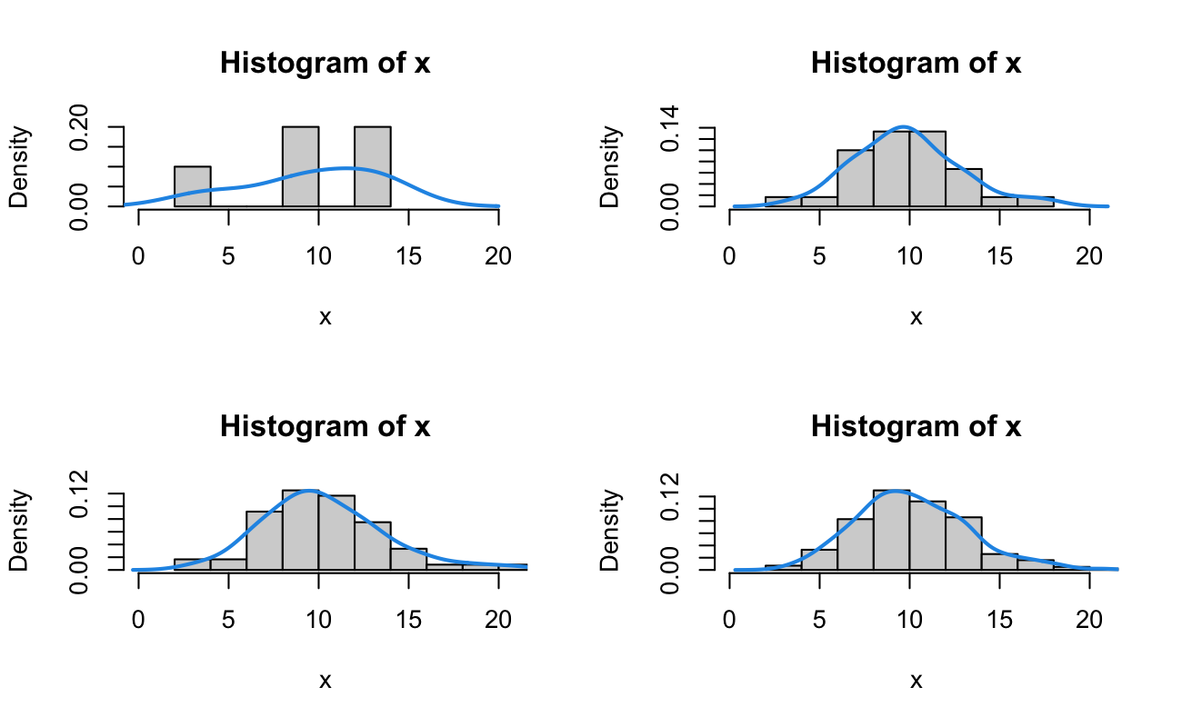
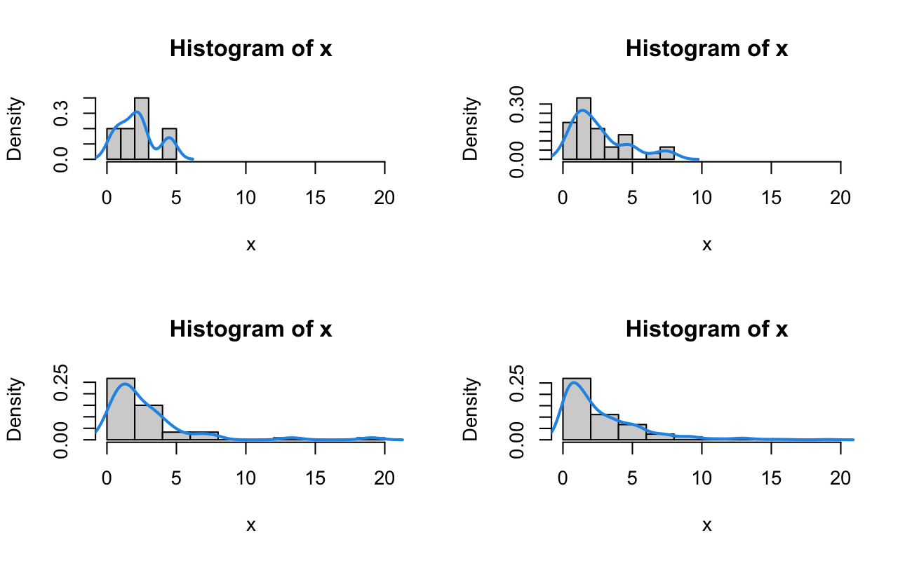
Let’s generate some random data. We continue our “clinic” example, but this time we want to know how long it will take us to have 3 patients within one hour. Our motivation could be as follows: we only have three nurses working in the clinic, and so we want to know how long we have to wait before all three nurses have a patient to see. We generate 7 “waiting times” until the third patient walks in. For a single experiment, that is, when we first open the clinic, how long will we have to wait for the third patient to arrive? Let’s assume the same rate of \(\lambda = 5\) for one hour (just like we used in the Exponential and Poisson lessons), and we are waiting for event \(\alpha = 3\). We can generate data (in fractional hours) by
So, for these 7 independent trials where the waiting times \(T\) have an identical Gamma distribution with rate of 5 patients per hour, we wait 54.3, 32.5, 24.1, 54.5, 46.7, 43.5, 85.6 minutes to see the third patient.
Based on the sample we saw above, \(\bar{x}\) = 0.813 and \(s^2\) = 0.108. We then solve the following system: \[
\begin{aligned}
(1)&\qquad \bar{x} = \frac{\alpha}{\lambda} \Rightarrow \alpha = \bar{x}\lambda, \\
(2)&\qquad s^2 = \frac{\alpha}{\lambda^2} \Rightarrow \alpha = s^2\lambda^2.
\end{aligned}
\] So, \[
\bar{x}\lambda = s^2\lambda^2 \Rightarrow \bar{x} = s^2\lambda \Rightarrow \hat{\lambda}_{MoM} = \frac{\bar{x}}{s^2}.
\] Substituting this back into Equation (1), we have \[
\hat{\alpha}_{MoM} = \bar{x}\left[\frac{\bar{x}}{s^2}\right] = \frac{\bar{x}^2}{s^2}.
\] We calculate these from the data we “observed”:
Thus, our Method of Moments estimates are \(\hat{\lambda}_{MoM}\) = 7.551 and \(\hat{\alpha}_{MoM}\) = 6.136, while the true values were \(\lambda = 5\) and \(\alpha = 3\). In my simulations, the Method of Moments estimates didn’t get “good” until I had over 70 samples.
7.9 Maximum Likelihood Estimators
Assume that we have observed a sample of waiting times \(\textbf{t} = (t_1, t_2, \ldots, t_n)\) which were generated from a Gamma waiting process.
The (much) simpler case is when we know how many “events”, \(\alpha\), the observers were waiting for when they recorded \(\textbf{t}\). If \(\alpha\) is known, then \[
\begin{aligned}
\ell(\alpha,\lambda|\textbf{t}) &= n\alpha\log(\lambda) - n\log(\Gamma(\alpha)) + (\alpha - 1) \sum_{i = 1}^n \log(t_i) - n\lambda\bar{t} \\
\Longrightarrow \frac{\partial}{\partial\lambda} \ell(\alpha,\lambda|\textbf{t}) &= \frac{\partial}{\partial\lambda} \left[ n\alpha\log(\lambda) - n\log(\Gamma(\alpha)) + (\alpha - 1) \sum_{i = 1}^n \log(t_i) - n\lambda\bar{t} \right] \\
&= \frac{n\alpha}{\lambda} - 0 + 0 - n\bar{t} \\
\Longrightarrow 0 &\overset{\text{set}}{=} \frac{n\alpha}{\hat{\lambda}} - n\bar{t} \\
\Longrightarrow n\bar{t} &= \frac{n\alpha}{\hat{\lambda}} \\
\Longrightarrow \bar{t} &= \frac{\alpha}{\hat{\lambda}} \\
\Longrightarrow \hat{\lambda} &= \frac{\alpha}{\bar{t}}.
\end{aligned}
\] Moreover, we see quickly that the second derivative with respect to \(\lambda\) is \(-n\alpha\lambda^{-2} < 0\), so \(\hat{\lambda}\) maximizes the likelihood. If we knew that the observers who collected the data were recording waiting times until they had observed three successes, then we can estimate the rate: \(\hat{\lambda}_{MLE}\) = 3.691.
7.9.3 MLE for \(\alpha\)
If \(\alpha\) is unknown, we start with the same log-likelikelihood as above, but quickly run out of “algebra” to do: \[
\begin{aligned}
\ell(\alpha,\lambda|\textbf{t}) &= n\alpha\log(\lambda) - n\log(\Gamma(\alpha)) + (\alpha - 1) \sum_{i = 1}^n \log(t_i) - n\lambda\bar{t} \\
\Longrightarrow \frac{\partial}{\partial\alpha} \ell(\alpha,\lambda|\textbf{t}) &= \frac{\partial}{\partial\alpha} \left[ n\alpha\log(\lambda) - n\log(\Gamma(\alpha)) + (\alpha - 1) \sum_{i = 1}^n \log(t_i) - n\lambda\bar{t} \right] \\
&= n\log(\lambda) - n \frac{\partial}{\partial\alpha} \log(\Gamma(\alpha)) + \sum_{i = 1}^n \log(t_i) \\
&= n\log(\lambda) - n \frac{\partial}{\partial\alpha} \log(\Gamma(\alpha)) + n\overline{\log(t)},
\end{aligned}
\] where \(\overline{\log(t)}\) denotes the average of the natural logarithms of the observed times (it’s still a fixed quantity).
7.9.3.1 Regular Solution
When we set this equal to 0, we have two “routes” to estimate a solution for this problem. The first option uses the derivative of the natural logarithm of the Gamma Function, known as the Digamma Function11, and symbolized \(\varphi(\alpha)\). Then, \[
\begin{aligned}
0 &\overset{\text{set}}{=} n\log(\lambda) - n \frac{\partial}{\partial\alpha} \log(\Gamma(\alpha)) + n\overline{\log(t)} \\
&= \log(\lambda) - \varphi(\alpha) + \overline{\log(t)} \\
\Longrightarrow \varphi(\alpha) &= \log(\lambda) + \overline{\log(t)}.
\end{aligned}
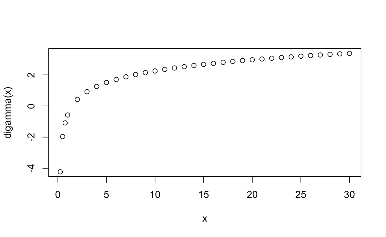
\] This would require numerical routines to estimate a solution for \(\hat{\alpha}\). Here’s what the Digamma function looks like:
Code
x <-c(0.25, 0.5, 0.75, 1:30)plot(x = x,y =digamma(x))
So, we have that \(\hat{\lambda} = \alpha/\bar{t}\) and \(\varphi(\hat{\alpha}) = \log(\lambda) + \overline{\log(t)}\). That’s two equations and two unknowns, which we might be able to approximate a solution to.
7.9.3.2 Another (Probably Bad) Option
The second option is a work in progress, and I’m not sure it’s even viable. I’m including it here to show some of my thought process. We will leave the derivative with respect to \(\alpha\) and work with the resulting differential equation. Thankfully this differential equation is in the form \(y^{\prime} = C\) with respect to \(\alpha\): \[
\begin{aligned}
0 &\overset{\text{set}}{=} n\log(\lambda) - n \frac{\partial}{\partial\alpha} \log(\Gamma(\alpha)) + n\overline{\log(t)} \\
\Longrightarrow \frac{\partial}{\partial\alpha} \log(\Gamma(\alpha)) &= \log(\lambda) + \overline{\log(t)} \\
\Longrightarrow \log(\Gamma(\alpha)) &= \alpha\left( \log(\lambda) + \overline{\log(t)} \right) + C.
\end{aligned}
\] We also need numerical routines to solve this. But the difficult part here is that we know very little about what kind of boundary conditions the Gamma Distribution has. We know that when \(\alpha = 1\), the Gamma Distribution reduces back to the Exponential Distribution, and we know that the MLE for \(\lambda\) in the Exponential Distribution is \((\bar{t})^{-1}\), which we can substitute in to solve for C:12\[
\begin{aligned}
\log(\Gamma([1])) &= [1]\left( \log(\bar{t}^{-1}) + \overline{\log(t)} \right) + C \\
\Longrightarrow \log(1) &= \log(\bar{t}^{-1}) + \overline{\log(t)} + C \\
\Longrightarrow 0 &= -\log(\bar{t}) + \overline{\log(t)} + C \\
\Longrightarrow C &= \log(\bar{t}) - \overline{\log(t)}.
\end{aligned}
\] Therefore, we would use a numerical routine to find \(\hat{\alpha}\) as the solution to \[
\begin{aligned}
\log(\Gamma(\alpha)) &= \alpha\left( \log(\lambda) + \overline{\log(t)} \right) + \log(\bar{t}) - \overline{\log(t)} \\
&= \alpha\left( -\log(\bar{t}) + \overline{\log(t)} \right) + \log(\bar{t}) - \overline{\log(t)} \\
&= -\alpha\left( \log(\bar{t}) - \overline{\log(t)} \right) + \log(\bar{t}) - \overline{\log(t)} \\
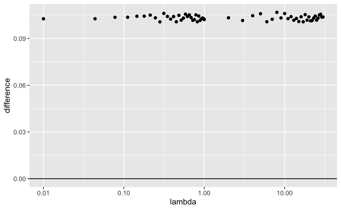
&= -\alpha K + K \\
&= K(1 - \alpha),
\end{aligned}
\] where \(K = \log(\bar{t}) - \overline{\log(t)}\). Now what does this \(K\) look like? For fixed \(\alpha\), we can generate vectors \(\textbf{t}\) with increasing \(\lambda\). Then we can plot the values of \(\log(\bar{t}) - \overline{\log(t)}\) (on a log scale for \(\lambda\)).