# Installing Required Packages
# intsall.packages("foreign")
# intsall.packages("skimr")
# intsall.packages("gtsummary")
# intsall.packages("GGally")
# install.packages("glmnet")
# install.packages("car")
# intsall.packages(tidyverse)

# Loading Required Packages
library(foreign)
library(skimr)
library(gtsummary)
library(GGally)
library(glmnet)
library(car)
library(tidyverse)35 Elastic Net Regression Model
35.1 Libraries for the lessons
For this chapter, we will be using the following packages
-
foreign: for reading SPSS and STATA datasets -
skimr: for summaries the datasets -
gtsummary: for coming up with nice tables for results and plotting the graphs -
GGally: for plotting the pairs graphs -
glmnet: ridge regression model -
car: for finding vif -
tidyverse: a general and powerful package for data transformation
These are loaded as follows using the function library(),
35.2 Introduction to Elastic Net Regression
In multiple linear regression analysis, it is not uncommon for specific problems to arise during the analysis. One of them is the problem of multicollinearity. Multicollinearity is a condition that appears in multiple regression analysis when one independent variable is correlated with another independent variable. Multicollinearity can create inaccurate estimates of the regression coefficients, inflate the standard errors of the regression coefficients, deflate the partial t-tests for theregression coefficients, give false, nonsignificant, p-values, and degrade the predictability of the model. Multicollinearity is a serious problem, where in cases of high multicollinearity, it results in making inaccurate decisions or increasing the chance of accepting the wrong hypothesis. Therefore it is very important to find the most suitable method to deal with multicollinearity. There are several ways to detect the presence of multicollinearity including looking at the correlation between independent variables and using the Variance Inflation Factor (VIF). As for the method to overcome the problem of multicollinearity, one way is by shrinking the estimated coefficients. The shrinkage method is often referred to as the regularization method. The regularization method can shrink the parameters to near zero relative to the least squares estimate. The regularization methods that are often used are Regression Ridge, Least Absolute Shrinkage and Selection Operator (LASSO), and Elastic-Net. Ridge Regression(RR) is a technique to stabilize the value of the regression coefficient due to multicollinearity problems. By adding a degree of bias to the regression estimate, RR reduces the standard error and obtains a more accurate estimate of the regression coefficient than the OLS. Meanwhile, LASSO and Elastic-Net overcome the problem of multicollinearity by reducing the regression coefficients of the independent variables that have a high correlation close to zero or exactly zero.
35.3 Mathematical Formulation of the Model
One method that can be used to estimate parameters is Ordinary Least Squares (OLS). This method requires the absence of multicollinearity between independent variables. If the independent variable has multicollinearity, the estimate of the regression coefficient may be imprecise. This method is used to estimate \(\beta\) by minimizing the sum of squared errors. If the data consists of n observations \([{y_i, x_i}]^n_{i=1}\) and each observation i includes a scalar response \(y_i\) and a vector of p predictors (regressors) \(x_{ij}\) for j = 1, …, m, a multiple linear regression model can be written as n the matrix form the model as \(Y = X \beta + \epsilon\) where \(Y_{n \times 1}\) is the vector dependent variable, \(X_{n \times m}\) represents the explanatory variables, \(\beta_{m \times 1}\) is the regression coefficients to be estimated, and \(\epsilon_{m \times 1}\) represents the errors or residuals. \(\hat\beta_{OLS} = (X^T X)^{-1} X^T Y\) is estimated regression coefficients using OLS by minimizing the squared distances between the observed and the predicted dependent variable. To have unbiased OLS estimation of the model, some assumptions should be satisfied. Those assumptions are that the errors have an expected value of zero, that the independent variables are non-random, that the independent variables are linearly independent (non-multicollinearity), that the disturbance are homoscedastic and not autocorrelated. If the independent variables have multicollinearity the estimates of coefficient regression may be imprecise.
35.3.1 Ridge Regression
Ridge regression introduced by Horel (1962) is one method for deal with multicollinearity problems. The ridge regression technique is based on addition the ridge parameter (\(\lambda\)) to the diagonal of the \(X^T X\) matrix forms a new matrix \((X^T X + \lambda I)\). is called ridge regression because diagonal one in the correlation matrix can be described as ridge Hoerl and Kennard (1970). The ridge regression coefficients estimator is \[
\hat\beta_R = (X^T X + \lambda I)^{-1} X^T Y, \lambda \geq 0
\] when \(\lambda = 0\), the ridge estimator become as the OLS. If \(\lambda > 0\) the ridge estimator will be biased against the \(\hat\beta_{OLS}\) but tends to be more accurate than the least squares estimator. Ridge regression can also be written in Lagrangian form: \[
\hat\beta_{\text{RIDGE}} = \arg \min_{\beta}||y - X\beta||^2_2 + \lambda||\beta||^2_2
\] where \(||y - X\beta||^2_2 = \sum^n_{i=1}(y_i - x^T_i\beta)^2\) is norm loss function (i.e. residual sum of squares), \(x^T_i\) is the i-th row of X, \(||\beta||^2_2 = \sum^p_{j=1}\beta^2_j\) is the penalty on \(\beta\), and \(\lambda \geq 0\) is the tuning parameter which regulates the strength of the penalty by determining the relative importance of the data-dependet empirical error and penalty term. Ridge regression has the ability to solve problems multicollinearity by limiting the estimated coefficients, hence, it reduces the estimator’s variance but introduces some bias.
35.3.2 Least Absolute Shrinkage and Selection Operator
Least Absolute Shrinkage and Selection Operator (LASSO) introduced by Tibshirani (1996) is a method that aims to reduce the regression coefficients of independent variables that have a high correlation with errors to exactly zero or close to zero. LASSO regression can also be written in Lagrangian form: \[ \hat\beta_{\text{LASSO}} = \arg \min_{\beta}||y - X\beta||^2_2 + \lambda||\beta||_1 \] where \(||\beta||_1 = \sum^p_{j=1}|\beta_j|\) is the penalty on \(\beta\). with the condition \(||\beta||_1 \leq \lambda\), where \(\lambda\) is a tuning parameter that controls the shrinkage of the LASSO coefficient with \(\lambda \geq 0\). If \(\lambda < \lambda_0\) with \(\lambda_0 = ||\hat\beta_j||_1\) it will cause the shrinkage coefficient to approach zero or exactly zero, so LASSO helps as a variable selection. Like ridge, the absolute value penalty of the LASSO coefficient introduces shrinkage towards zero. However, on ridge regression, some of the coefficients are not shrinks to exactly zero.
35.3.3 Elastic Net
According to Zou and Hastie (2005), the Elastic-Net method can shrink the regression coefficient exactly to zero, besides that this method can also perform variable selection simultaneously with Elastic-Net penalties which are written as follows: \[
\sum^p_{j=1}[\alpha |\beta_j| + (1 - \alpha)\beta^2_j]
\] with \(\alpha = \frac{\lambda_1}{\lambda_1 + \lambda_2},0 \leq \alpha \leq 1\). The coefficient estimator on Elastic-Net can be written as follows: \[
\hat\beta_{\text{Elastic-net}} = \arg \min_{\beta}||y - X\beta||^2_2 + \lambda_2||\beta||^2_2 + \lambda_1||\beta||_1
\] Elastic-Net can be used to solve problems from LASSO. Where the LASSO Regression has disadvantages include; when p > n then LASSO only chooses n variables included in the model, if there is a set of variables with high correlation, then LASSO only tends to choose one variable from the group and doesn’t care which one is selected, and when p < n, LASSO performance is dominated by Ridge Regression. Multicollinearity is the existence of a linear relationship between independent variables, where multicollinearity can occur in either some or all of the independent variables in the multiple linear regression model. One way to detect multicollinearity is to use the Variation Inflation Factor (VIF). VIF value can be calculated by the following formula: \[
\text{VIF}_j = \frac{1}{1 - R^2_j}
\] if the VIF value > 10, it can be concluded significantly that there is multicollinearity between the independent variables and one way to overcome multicollinearity is using the Ridge Regression, LASSO and Elastic-Net.
35.4 Example
To demostrate the Elastic net regression, we will use coronary.dta (https://github.com/drkamarul/multivar_data_analysis/tree/main/data) dataset in STATA format. The dataset contains the total cholesterol level, their individual characteristics and intervention groups in a hypothetical clinical trial. The dataset contains 200 observations for nine variables:
-
id: Subjects’ ID. -
cad: Coronary artery disease status (categorical) {no cad, cad}. -
sbp: Systolic blood pressure in mmHg (numerical). -
dbp: Diastolic blood pressure in mmHg (numerical). -
chol: Total cholesterol level in mmol/L (numerical). -
age: Age in years (numerical). -
bmi: Body mass index (numerical). -
race: Race of the subjects (categorical) {malay, chinese, indian}. -
gender: Gender of the subjects (categorical) {woman, man}.
35.4.1 Exploring the data
The dataset is loaded as follows,
    id    cad sbp dbp   chol age      bmi    race gender
1    1 no cad 106  68 6.5725  60 38.90000  indian  woman
2   14 no cad 130  78 6.3250  34 37.80000   malay  woman
3   56 no cad 136  84 5.9675  36 40.50000   malay  woman
4   61 no cad 138 100 7.0400  45 37.60000   malay  woman
5   62 no cad 115  85 6.6550  53 40.30000  indian    man
6   64 no cad 124  72 5.9675  43 37.60000   malay    man
7   69    cad 110  80 4.4825  44 34.28411   malay    man
8  108 no cad 112  70 5.4725  50 40.90000 chinese  woman
9  112 no cad 138  85 7.4525  43 41.20000 chinese  woman
10 134 no cad 104  70 6.4350  48 41.00000 chinese    man
35.4.1.1 Structure of the dataset
str(coronary)'data.frame': 200 obs. of 9 variables:
$ id : num 1 14 56 61 62 64 69 108 112 134 ...
$ cad : Factor w/ 2 levels "no cad","cad": 1 1 1 1 1 1 2 1 1 1 ...
$ sbp : num 106 130 136 138 115 124 110 112 138 104 ...
$ dbp : num 68 78 84 100 85 72 80 70 85 70 ...
$ chol : num 6.57 6.33 5.97 7.04 6.66 ...
$ age : num 60 34 36 45 53 43 44 50 43 48 ...
$ bmi : num 38.9 37.8 40.5 37.6 40.3 ...
$ race : Factor w/ 3 levels "malay","chinese",..: 3 1 1 1 3 1 1 2 2 2 ...
$ gender: Factor w/ 2 levels "woman","man": 1 1 1 1 2 2 2 1 1 2 ...
- attr(*, "datalabel")= chr "Written by R. "
- attr(*, "time.stamp")= chr ""
- attr(*, "formats")= chr [1:9] "%9.0g" "%9.0g" "%9.0g" "%9.0g" ...
- attr(*, "types")= int [1:9] 100 108 100 100 100 100 100 108 108
- attr(*, "val.labels")= chr [1:9] "" "cad" "" "" ...
- attr(*, "var.labels")= chr [1:9] "id" "cad" "sbp" "dbp" ...
- attr(*, "version")= int 7
- attr(*, "label.table")=List of 3
..$ cad : Named int [1:2] 1 2
.. ..- attr(*, "names")= chr [1:2] "no cad" "cad"
..$ race : Named int [1:3] 1 2 3
.. ..- attr(*, "names")= chr [1:3] "malay" "chinese" "indian"
..$ gender: Named int [1:2] 1 2
.. ..- attr(*, "names")= chr [1:2] "woman" "man"35.4.1.2 Summary
skim(coronary)| Name | coronary |
| Number of rows | 200 |
| Number of columns | 9 |
| _______________________ | |
| Column type frequency: | |
| factor | 3 |
| numeric | 6 |
| ________________________ | |
| Group variables | None |
Variable type: factor
| skim_variable | n_missing | complete_rate | ordered | n_unique | top_counts |
|---|---|---|---|---|---|
| cad | 0 | 1 | FALSE | 2 | no : 163, cad: 37 |
| race | 0 | 1 | FALSE | 3 | mal: 73, chi: 64, ind: 63 |
| gender | 0 | 1 | FALSE | 2 | wom: 100, man: 100 |
Variable type: numeric
| skim_variable | n_missing | complete_rate | mean | sd | p0 | p25 | p50 | p75 | p100 | hist |
|---|---|---|---|---|---|---|---|---|---|---|
| id | 0 | 1 | 2218.28 | 1411.69 | 1.00 | 901.50 | 2243.50 | 3346.75 | 4696.00 | ▇▅▇▆▅ |
| sbp | 0 | 1 | 130.18 | 19.81 | 88.00 | 115.00 | 126.00 | 144.00 | 187.00 | ▂▇▅▃▁ |
| dbp | 0 | 1 | 82.31 | 12.90 | 56.00 | 72.00 | 80.00 | 92.00 | 120.00 | ▂▇▆▃▁ |
| chol | 0 | 1 | 6.20 | 1.18 | 4.00 | 5.39 | 6.19 | 6.89 | 9.35 | ▅▇▇▃▂ |
| age | 0 | 1 | 47.33 | 7.34 | 32.00 | 42.00 | 47.00 | 53.00 | 62.00 | ▃▇▇▆▃ |
| bmi | 0 | 1 | 37.45 | 2.68 | 28.99 | 36.10 | 37.80 | 39.20 | 45.03 | ▁▂▇▆▁ |
35.4.1.3 Descriptives
coronary %>%
tbl_summary()| Characteristic | N = 2001 |
|---|---|
| id | 2,244 (902, 3,347) |
| cad | |
| no cad | 163 (82%) |
| cad | 37 (19%) |
| sbp | 126 (115, 144) |
| dbp | 80 (72, 92) |
| chol | 6.19 (5.39, 6.89) |
| age | 47 (42, 53) |
| bmi | 37.80 (36.10, 39.20) |
| race | |
| malay | 73 (37%) |
| chinese | 64 (32%) |
| indian | 63 (32%) |
| gender | |
| woman | 100 (50%) |
| man | 100 (50%) |
| 1 Median (IQR); n (%) | |
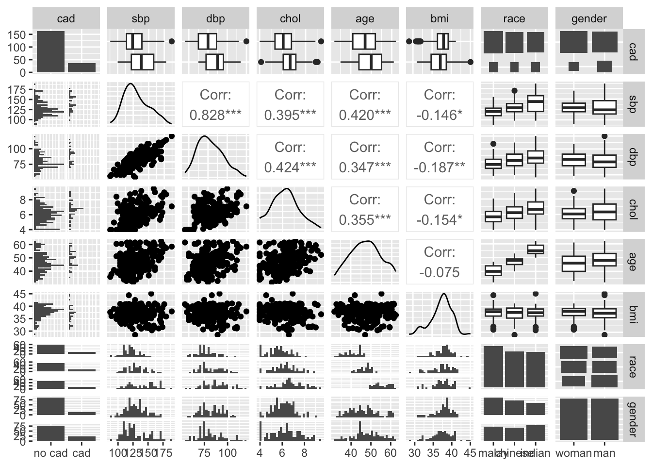
35.4.1.4 Pairs
35.4.1.5 Variance Inflation Factor (VIF)
The most common way to detect multicollinearity is by using the variance inflation factor (VIF), which measures the correlation and strength of correlation between the predictor variables in a regression model.
The value for VIF starts at 1 and has no upper limit. A general rule of thumb for interpreting VIFs is as follows:
- A value of 1 indicates there is no correlation between a given predictor variable and any other predictor variables in the model.
- A value between 1 and 5 indicates moderate correlation between a given predictor variable and other predictor variables in the model, but this is often not severe enough to require attention.
- A value greater than 5 indicates potentially severe correlation between a given predictor variable and other predictor variables in the model. In this case, the coefficient estimates and p-values in the regression output are likely unreliable.
35.5 Fitting the regression mode
We are interested in knowing the relationship between blood pressure (SBP and DBP), age, and BMI as the predictors and the cholesterol level (outcome).
35.5.1 Ridge regression model
In R, we can use ridge regression using several packages, with glmnet being one of the most popular.
# X and y datasets
X <- coronary %>%
  select(-id, -cad, -chol, -race, -gender) %>%
  as.matrix()
X_train <- X[1:150,]
X_test <- X[151:200,]

y <- coronary %>%
  select(chol) %>%
  as.matrix()
y_train <- y[1:150,]
y_test <- y[151:200,]

# Fit the model
ridge_model <- glmnet(X_train, y_train, alpha = 0)

# Cross-validation
cv_ridge <- cv.glmnet(X_train, y_train, alpha = 0)

# Optimal lambda
ridge_best_lambda <- cv_ridge$lambda.min

# Refit the model with the best lambda
ridge_model_best <- glmnet(X_test, y_test, alpha = 0, lambda = ridge_best_lambda)

# Coefficients
coef(ridge_model_best)
5 x 1 sparse Matrix of class "dgCMatrix"
s0
(Intercept) 4.833796427
sbp 0.016509767
dbp 0.010086680
age -0.002821509
bmi -0.043286358# Predict values using the fitted model
ridge_pred <- predict(ridge_model_best, newx = X_test)
# Calculate RMSE
ridge_rmse <- sqrt(mean((ridge_pred - y_test)^2))
print(ridge_rmse)[1] 1.00202# Manually predict values using the fitted model and RMSE
ridge_pred_manual <- as.matrix(cbind(1, X_test)) %*% coef(ridge_model_best)
sqrt(mean((y_test - ridge_pred_manual)^2))[1] 1.0020235.5.2 LASSO Regression
# Fit the lasso regression model
lasso_model <- glmnet(X_train, y_train, alpha = 1) # alpha = 1 for lasso regression

# Cross-validation
cv_lasso <- cv.glmnet(X_train, y_train, alpha = 1)

# Optimal lambda
lasso_best_lambda <- cv_lasso$lambda.min # Lambda value with miniumum cross-validated error

# Refit the model with the best lambda
lasso_model_best <- glmnet(X_test, y_test, alpha = 1, lambda = lasso_best_lambda)

coef(lasso_model_best)
5 x 1 sparse Matrix of class "dgCMatrix"
s0
(Intercept) 4.297403627
sbp 0.018368084
dbp 0.004110394
age .
bmi -0.025892099# Predict using the best lambda
lasso_pred <- predict(lasso_model_best, newx = X_test)
# Calculate RMSE
lasso_rmse <- sqrt(mean((lasso_pred - y_test)^2))
print(lasso_rmse)[1] 1.005208# Manually predict values using the fitted model and RMSE
lasso_pred_manual <- as.matrix(cbind(1, X_test)) %*% coef(lasso_model_best)
sqrt(mean((y_test - lasso_pred_manual)^2))[1] 1.00520835.5.3 Elastic Net Regresssion
# Fit the elastic net regression model
elastic_net_model <- glmnet(X_train, y_train, alpha = 0.5) # alpha = 0.5 for elastic net

cv_elastic <-  cv.glmnet(X_train, y_train, alpha = 0.5)

elastic_best_lambda <-  cv_elastic$lambda.min

elastic_model_best <- glmnet(X_test, y_test, alpha = 0.5, lambda = elastic_best_lambda)

coef(elastic_model_best)
5 x 1 sparse Matrix of class "dgCMatrix"
s0
(Intercept) 4.522796707
sbp 0.018225191
dbp 0.006431528
age .
bmi -0.036498892# Predict using the best lambda
elastic_pred <- predict(elastic_model_best, newx = X_test)
# Calculate RMSE
elastic_rmse <- sqrt(mean((elastic_pred - y_test)^2))
print(elastic_rmse)[1] 1.002382# Manually predict values using the fitted model and RMSE
elastic_pred_manual <- as.matrix(cbind(1, X_test)) %*% coef(elastic_model_best)
sqrt(mean((y_test - elastic_pred_manual)^2))[1] 1.00238235.6 Results
35.6.1 Coefficients
c1 <- coef(ridge_model_best) %>% as.matrix()
c2 <- coef(lasso_model_best) %>% as.matrix()
c3 <- coef(elastic_model_best) %>% as.matrix()

coef <- cbind(c1, c2, c3)
colnames(coef) <- c("Ridge", "LASSO", "Elastic Net")
print(coef)
Ridge LASSO Elastic Net
(Intercept) 4.833796427 4.297403627 4.522796707
sbp 0.016509767 0.018368084 0.018225191
dbp 0.010086680 0.004110394 0.006431528
age -0.002821509 0.000000000 0.000000000
bmi -0.043286358 -0.025892099 -0.03649889235.6.2 RMSE
35.7 Summary
In this lecture, we went through the basic multicollinearity problem of liner regression model and trying yo solve it. We discussed different methods about this. We can solve the multicollinearity problem using ridge, LASSO and Elastic-net. We can also compare between them using both simulated data and real data based on different criteria. And, based on those we can say that which one can perform better than others.
Hoerl, Arthur E, and Robert W Kennard. 1970. “Ridge Regression: Biased Estimation for Nonorthogonal Problems.” Technometrics 12 (1): 55–67.
Horel, AE. 1962. “Application of Ridge Analysis to Regression Problems.” Chemical Engineering Progress 58: 54–59.
Tibshirani, Robert. 1996. “Regression Shrinkage and Selection via the Lasso.” Journal of the Royal Statistical Society Series B: Statistical Methodology 58 (1): 267–88.
Zou, Hui, and Trevor Hastie. 2005. “Regularization and Variable Selection via the Elastic Net.” Journal of the Royal Statistical Society Series B: Statistical Methodology 67 (2): 301–20.