#install.packages("ggstatplot")
#install.packages("car")
#install.packages("rstatix")
#install.packages(tidyVerse)16 Two sample \(t\)-test
Explaining the Two sample \(t\)-test and how to run it in R
16.1 Two sample \(t\)-test
This is also called the independent sample t test. It is used to see whether the population means of two groups are equal or different. This test requires one variable which can be the exposure x and another variable which can be the outcome y. If there are more than two groups, Analysis of Variance (ANOVA) would be more suitable. If data is nonparametric then an alternative test to use would be the Mann Whitney U test. Cressie, N.A., 1986
There are two types of independent t tests: the first is the Student’s t test, which assumes the variance of the two groups is equal, and the second being the Welch’s t test (default in R), which assumes the variance in the two groups is different.
In this article we will be discussing the Student’s t test.
16.1.1 Assumptions
Measurements for one observation do not affect measurements for any other observation (assumes independence).
Data values in dependent variable are continuous.
Data in each group are normally distributed.
The variances for the two independent groups are equal in the Student’s t test.
There should be no significant outliers.
16.1.2 Hypotheses
\((H_0)\): the mean of group A \((m_A)\) is equal to the mean of group B \((m_B)\)- two tailed test.
\((H_0)\): \((m_A)\ge (m_B)\)- one tailed test.
\((H_0)\): \((m_A)\le (m_B)\)- one tailed test.
The corresponding alternative hypotheses would be as follows:
- \((H_1)\): \((m_A)\neq(m_B)\)- two tailed test.
- \((H_1)\): \((m_A)<(m_B)\)- one tailed test.
- \((H_1)\): \((m_A)> (m_B)\)- one tailed test.
16.1.3 Statistical hypotheses formula
For the Student’s t test which assumes equal variance, here is an example of how the |t| statistic may be calculated using groups A and B:
\(t ={ {m_{A} - m_{B}} \over \sqrt{ {S^2 \over n_{A} } + {S^2 \over n_{B}} }}\)
This can be described as the sample mean difference divided by the sample standard deviation of the sample mean difference where:
\(m_A\) and \(m_B\) are the mean values of A and B,
\(n_A\) and \(n_B\) are the size of group A and B,
\(S^2\) is the estimator for the pooled variance, with the degrees of freedom (df) = \(n_A + n_B - 2\),
and \(S^2\) is calculated as follows:
\(S^2 = { {\sum{ (x_A-m_{A})^2} + \sum{ (x_B-m_{B})^2}} \over {n_{A} + n_{B} - 2 }}\)
What if the data is not independent?
If the data is not independent such as paired data in the form of matched pairs which are correlated, we use the paired t test. This test checks whether the means of two paired groups are different from each other. It is usually applied in clinical trial studies with a “before and after” or case control studies with matched pairs. For this test we only assume the difference of each pair to be normally distributed (the paired groups are the ones important for analysis) unlike the independent t test which assumes that data from both samples are independent and variances are equal. Xu, M., 2017
16.1.4 Example
16.1.4.1 Prerequisites
-
tidyverse: data manipulation and visualization. -
rstatix: providing pipe friendly R functions for easy statistical analysis. -
car: providing variance tests.
16.1.4.2 Dataset
This example dataset sourced from kaggle was obtained from surveys of students in Math and Portuguese classes in secondary school. It contains demographic information on gender, social and study information.
# load the dataset
stu_math <- read_csv("../data/03_student-mat.csv")
Rows: 395 Columns: 33
── Column specification ────────────────────────────────────────────────────────
Delimiter: ","
chr (17): school, sex, address, famsize, Pstatus, Mjob, Fjob, reason, guardi...
dbl (16): age, Medu, Fedu, traveltime, studytime, failures, famrel, freetime...
ℹ Use `spec()` to retrieve the full column specification for this data.
ℹ Specify the column types or set `show_col_types = FALSE` to quiet this message.Checking the data
# check the data
glimpse(stu_math)
Rows: 395
Columns: 33
$ school <chr> "GP", "GP", "GP", "GP", "GP", "GP", "GP", "GP", "GP", "GP",…
$ sex <chr> "F", "F", "F", "F", "F", "M", "M", "F", "M", "M", "F", "F",…
$ age <dbl> 18, 17, 15, 15, 16, 16, 16, 17, 15, 15, 15, 15, 15, 15, 15,…
$ address <chr> "U", "U", "U", "U", "U", "U", "U", "U", "U", "U", "U", "U",…
$ famsize <chr> "GT3", "GT3", "LE3", "GT3", "GT3", "LE3", "LE3", "GT3", "LE…
$ Pstatus <chr> "A", "T", "T", "T", "T", "T", "T", "A", "A", "T", "T", "T",…
$ Medu <dbl> 4, 1, 1, 4, 3, 4, 2, 4, 3, 3, 4, 2, 4, 4, 2, 4, 4, 3, 3, 4,…
$ Fedu <dbl> 4, 1, 1, 2, 3, 3, 2, 4, 2, 4, 4, 1, 4, 3, 2, 4, 4, 3, 2, 3,…
$ Mjob <chr> "at_home", "at_home", "at_home", "health", "other", "servic…
$ Fjob <chr> "teacher", "other", "other", "services", "other", "other", …
$ reason <chr> "course", "course", "other", "home", "home", "reputation", …
$ guardian <chr> "mother", "father", "mother", "mother", "father", "mother",…
$ traveltime <dbl> 2, 1, 1, 1, 1, 1, 1, 2, 1, 1, 1, 3, 1, 2, 1, 1, 1, 3, 1, 1,…
$ studytime <dbl> 2, 2, 2, 3, 2, 2, 2, 2, 2, 2, 2, 3, 1, 2, 3, 1, 3, 2, 1, 1,…
$ failures <dbl> 0, 0, 3, 0, 0, 0, 0, 0, 0, 0, 0, 0, 0, 0, 0, 0, 0, 0, 3, 0,…
$ schoolsup <chr> "yes", "no", "yes", "no", "no", "no", "no", "yes", "no", "n…
$ famsup <chr> "no", "yes", "no", "yes", "yes", "yes", "no", "yes", "yes",…
$ paid <chr> "no", "no", "yes", "yes", "yes", "yes", "no", "no", "yes", …
$ activities <chr> "no", "no", "no", "yes", "no", "yes", "no", "no", "no", "ye…
$ nursery <chr> "yes", "no", "yes", "yes", "yes", "yes", "yes", "yes", "yes…
$ higher <chr> "yes", "yes", "yes", "yes", "yes", "yes", "yes", "yes", "ye…
$ internet <chr> "no", "yes", "yes", "yes", "no", "yes", "yes", "no", "yes",…
$ romantic <chr> "no", "no", "no", "yes", "no", "no", "no", "no", "no", "no"…
$ famrel <dbl> 4, 5, 4, 3, 4, 5, 4, 4, 4, 5, 3, 5, 4, 5, 4, 4, 3, 5, 5, 3,…
$ freetime <dbl> 3, 3, 3, 2, 3, 4, 4, 1, 2, 5, 3, 2, 3, 4, 5, 4, 2, 3, 5, 1,…
$ goout <dbl> 4, 3, 2, 2, 2, 2, 4, 4, 2, 1, 3, 2, 3, 3, 2, 4, 3, 2, 5, 3,…
$ Dalc <dbl> 1, 1, 2, 1, 1, 1, 1, 1, 1, 1, 1, 1, 1, 1, 1, 1, 1, 1, 2, 1,…
$ Walc <dbl> 1, 1, 3, 1, 2, 2, 1, 1, 1, 1, 2, 1, 3, 2, 1, 2, 2, 1, 4, 3,…
$ health <dbl> 3, 3, 3, 5, 5, 5, 3, 1, 1, 5, 2, 4, 5, 3, 3, 2, 2, 4, 5, 5,…
$ absences <dbl> 6, 4, 10, 2, 4, 10, 0, 6, 0, 0, 0, 4, 2, 2, 0, 4, 6, 4, 16,…
$ G1 <dbl> 5, 5, 7, 15, 6, 15, 12, 6, 16, 14, 10, 10, 14, 10, 14, 14, …
$ G2 <dbl> 6, 5, 8, 14, 10, 15, 12, 5, 18, 15, 8, 12, 14, 10, 16, 14, …
$ G3 <dbl> 6, 6, 10, 15, 10, 15, 11, 6, 19, 15, 9, 12, 14, 11, 16, 14,…In total there are 395 observations and 33 variables. We will drop the variables we do not need and keep the variables that will help us answer the following: Is there a difference between the finals grades of boys and girls in maths?
\(H_0\): There is no statistical difference between the final grades between boys and girls.
\(H_1\): There is a statistically significant differencehe in the final grades between the two groups.
Rows: 395
Columns: 2
$ sex <chr> "F", "F", "F", "F", "F", "M", "M", "F", "M", "M", "F", "F", "M", "…
$ G3  <dbl> 6, 6, 10, 15, 10, 15, 11, 6, 19, 15, 9, 12, 14, 11, 16, 14, 14, 10…
Summary statistics The dependent variable is continuous (grades=G3) and the independent variable is character but binary (sex).
# summarizing our data
 summary(math)
sex G3
Length:395 Min. : 0.00
Class :character 1st Qu.: 8.00
Mode :character Median :11.00
Mean :10.42
3rd Qu.:14.00
Max. :20.00 We see that data ranges from 0-20 with 0 being people who were absent and could not take the test therefore missing data.
Identifying outliers - Outliers can also be identified through boxplot.
# creating a boxplot to visualize the outliers (without removing score of zero)
ggplot(data = math) +
  aes(
    x = sex,
    y = G3
  ) +
  labs(
    title = "Boxplot to visualize the outlier",
    x  = "sex",
    y = "Maths Grades"
  ) +
  geom_boxplot()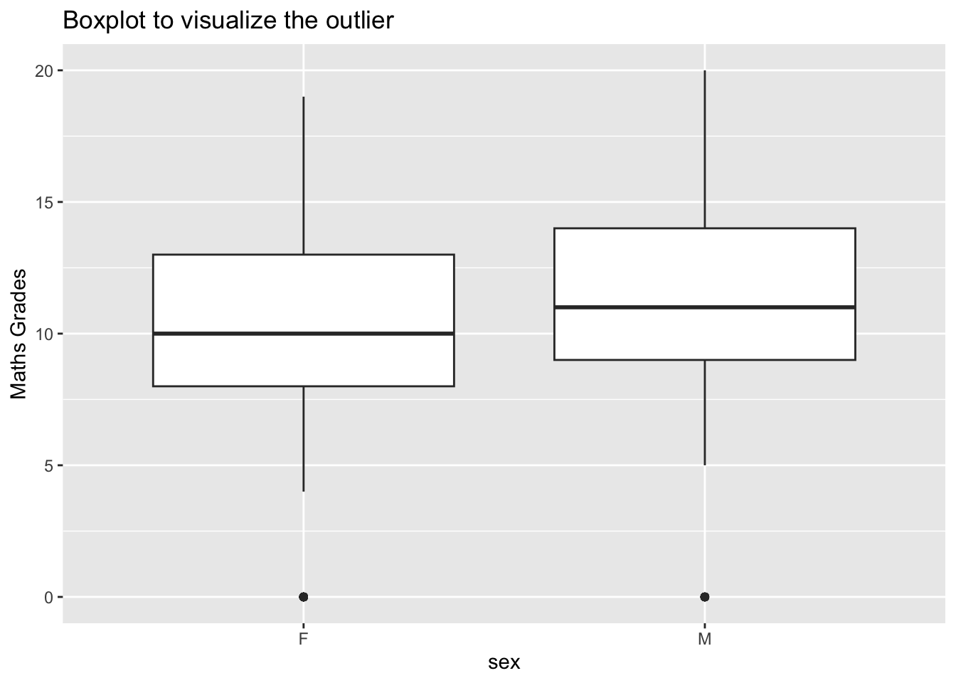
# creating a boxplot to visualize the data with no outliers
math2 <- math %>% filter(G3>0)
ggplot(data = math2) +
  aes(
    x = sex,
    y = G3
  ) +
  labs(
    title = "Boxplot without the outlier",
    x  = "sex",
    y = "Maths Grades"
  ) +
  geom_boxplot()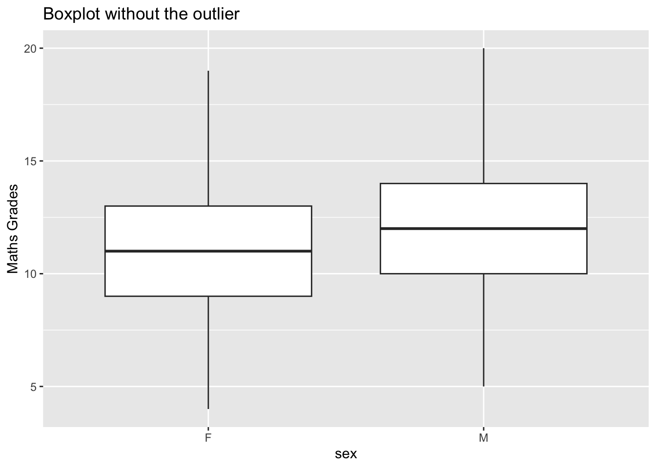
The second box plot shows us that there are no outliers as students with a score of zero have been removed. This score is not truly reflective of the performance between boys and girls as a grade of 0 may represent absence or other reasons for the test not been taken.
We remove the outliers before running the t test. However, other models can be considered such as the zero inflated model to differentiate those who truly got a 0 and those who were not present to take test.
# finding the mean for the groups with outliers (score of zero included)
mean(math$G3[math$sex=="F"])
[1] 9.966346mean(math$G3[math$sex=="M"])[1] 10.91444# finding the mean for the groups without outliers (score of zero not included)
mean(math2$G3[math2$sex=="F"])[1] 11.20541mean(math2$G3[math2$sex=="M"])[1] 11.86628The mean has increased slightly in both groups and the difference in mean has been decreased in both groups after removing the outliers.
Visualizing the data - We can use barplots to look at the difference in sample sizes between the groups and histograms check distribution of the data for normality.
sample_size <- table(math2$sex)
sample_size_df <- as.data.frame(sample_size)
colnames(sample_size_df) <- c("sex", "count")

# plotting bar plot to see the distribution in sample size
ggplot(data = sample_size_df) +
  aes(
    x = sex,
    y = count,
  ) +
  labs(
    title = "Distribution of sample size by sex",
    x = "Sex",
    y = "Number of students"
  ) +
  geom_bar(stat = "identity")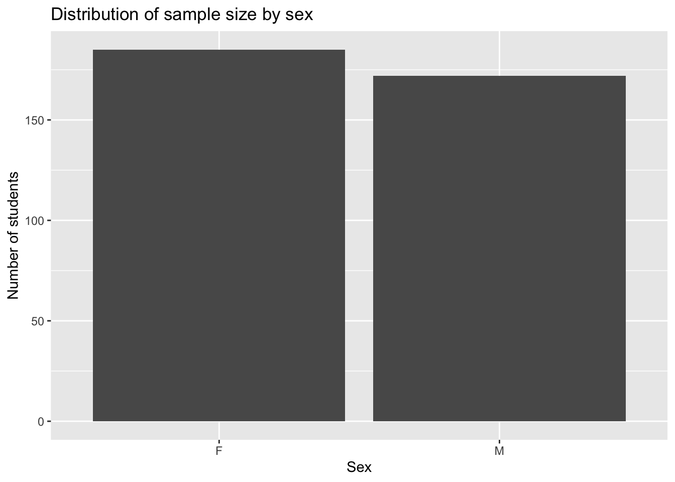
The bar graph shows that there are slightly more females in the sample than males.
# Histograms for data by groups

male = math2$G3[math2$sex == "M"]
female = math2$G3[math2$sex == "F"]

# plotting distribution for males
plotNormalHistogram(
  male,
  breaks= 20,
  xlim=c(0,20),
  main="Distribution of the grades for males ",
  xlab= "Math Grades"
  )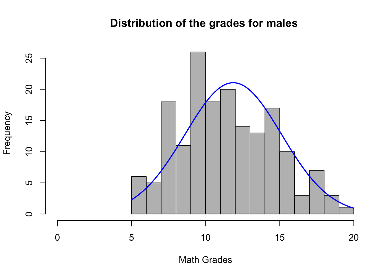
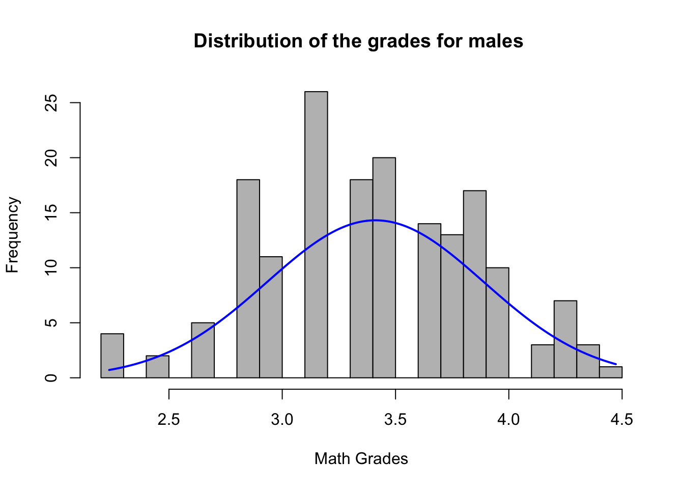
The final grades for males seem to be normally distributed. If it is difficult to be certain whether the data is normally distributed, the histogram of the square root transformed data can be plotted. It can help reveal underlying normality in skewed data by compressing the spread.
# plotting square root transformed distribution for males
plotNormalHistogram(
  sqrt(male),
  breaks= 20,
  main="Distribution of the grades for males ",
  xlab= "Math Grades"
  )
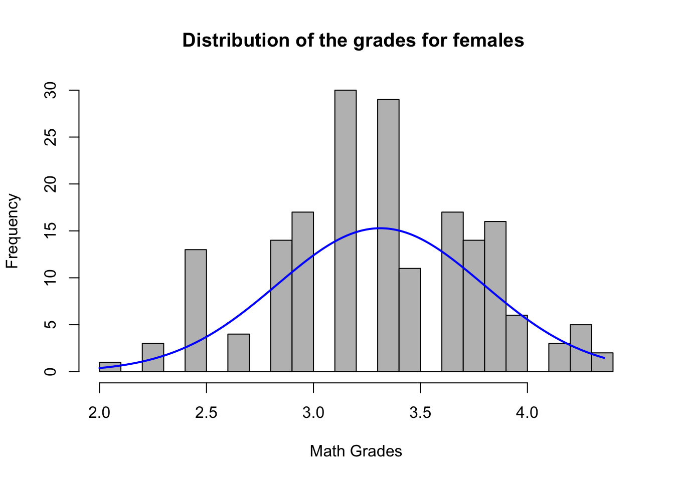
A highly skewed data might still not appear normal after square root transformation, so this is not a solution to a skewed data, but rather an approach to check normality more precisely.
# plotting distribution for females
plotNormalHistogram(
female,
breaks= 20,
xlim=c(0,20),
main="Distribution of the grades for females ",
xlab= "Math Grades"
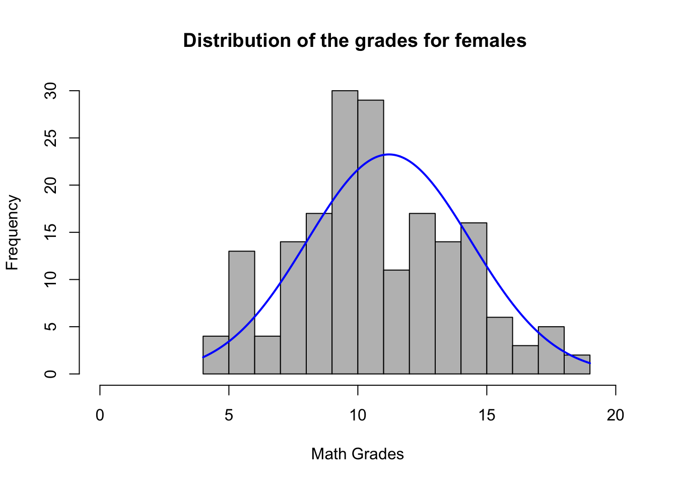
)
Similar to males, looking at the square root transformed distribution for females
# plotting square root transformed distribution for males
plotNormalHistogram(
  sqrt(female),
  breaks= 20,
  main="Distribution of the grades for females ",
  xlab= "Math Grades"
  )
Final grades for females also appear to be normally distributed. The final score across both is almost evenly distributed.
Check the equality of variances (homogeneity) - By looking at the two box plots above for two groups, it does not appear that the variances are different between the two groups.
We can use the Levene’s test or the Bartlett’s test to check for homogeneity of variances. The former is in the car library and the later in the rstatix library. If the variances are homogeneous, the p value will be greater than 0.05.
Other tests include F test 2 sided, Brown-Forsythe and O’Brien but we shall not cover these.
# running the Levene's test to check equal variance
math2 %>% levene_test(G3~sex)
# A tibble: 1 × 4
df1 df2 statistic p
<int> <int> <dbl> <dbl>
1 1 355 0.614 0.434#don't do this unless worried about the data# running the Bartlett's test to check equal variance
bartlett.test(G3~sex, data=math2)
    Bartlett test of homogeneity of variances

data:  G3 by sex
Bartlett's K-squared = 0.12148, df = 1, p-value = 0.7274
#don't do this unless worried about the dataThe p value is greater than 0.05 from both the test suggesting there is no difference between the variances of the two groups.
16.1.4.3 Assessment
Data is continuous(G3)
Data is independent (males and females are distinct and not the same individual)
Data is normally distributed. We might still want to do a square root transformation.
No significant outliers.
There are equal variances.
As the assumptions are met we go ahead to perform the Student’s \(t\)-test.
16.1.4.4 Performing the two-sample \(t\)-test
Since the default is the Welch t test we use the \(\color{blue}{\text{var.eqaul = TRUE }}\) code to signify a Student’s t test.
# perfoming the two sample t test
stat.test <- math2 %>%
  #mutate(sqrt_G3 = sqrt(G3)) %>%
  t_test(G3~ sex, var.equal=TRUE) %>%
  add_significance()
stat.test
# A tibble: 1 × 9
.y. group1 group2 n1 n2 statistic df p p.signif
<chr> <chr> <chr> <int> <int> <dbl> <dbl> <dbl> <chr>
1 G3 F M 185 172 -1.94 355 0.0531 ns stat.test$statistic t
-1.940477 If you decided to work with square root transformed data, you could use the mutate function to create the ‘sqrt_G3’ variable in the ‘stat.test’ dataset, which produces quite similar p-value and t test statistic.
The results are represented as follows;
y - dependent variable
group1, group 2 - compared groups (independent variables)
df - degrees of freedom
p - p value
gtsummary table of results
 math2 |>
  tbl_summary(
    by = sex,
    statistic =
      list(
        all_continuous() ~ "{mean} ({sd})")
    ) |>
   add_n() |>
  add_overall() |>
add_difference()| Characteristic | N | Overall, N = 3571 | F, N = 1851 | M, N = 1721 | Difference2 | 95% CI2,3 | p-value2 |
|---|---|---|---|---|---|---|---|
| G3 | 357 | 11.5 (3.2) | 11.2 (3.2) | 11.9 (3.3) | -0.66 | -1.3, 0.01 | 0.053 |
| 1 Mean (SD) | |||||||
| 2 Welch Two Sample t-test | |||||||
| 3 CI = Confidence Interval | |||||||
Interpretation of results
For the Student’s t test, the obtained t statistic of -1.940477 is greater than the critical value at 355 degree of freedom (n1+n2-2) i.e. -1.984, due to which it is not statistically significant. Also, the p-value is greater than alpha of 0.05, due to which we we fail to reject the null hypothesis and conclude that there is no statistical difference between the mean grades of boys and girls. (A significant |t| would be equal to -1.984 or smaller; or equal to 1.984 or greater).
Effect size Note: Effect size should only be calculated if the null hypothesis is rejected. We are showing how to do this for pedagogical reasons. In practice, we would not calculate an effect size because we fail to reject the null hypothesis.
Cohen’s d can be an used as an effect size statistic for the two sample t test. It is the difference between the means of each group divided by the pooled standard deviation.
\(d= {m_A-m_B \over SDpooled}\)
It ranges from 0 to infinity, with 0 indicating no effect where the means are equal. 0.5 means that the means differ by half the standard deviation of the data and 1 means they differ by 1 standard deviation. It is divided into small, medium or large using the following cut off points.
small 0.2-<0.5
medium 0.5-<0.8
large >=0.8
For the above test the following is how we can find the effect size;
# A tibble: 1 × 7
  .y.   group1 group2 effsize    n1    n2 magnitude
* <chr> <chr>  <chr>    <dbl> <int> <int> <ord>
1 G3    F      M       -0.206   185   172 small
The effect size is small d= -0.20.
In conclusion, a two-samples t-test showed that the difference was not statistically significant, t(355) = -1.940477, p < 0.0531, d = -0.20; where, t(355) is shorthand notation for a t-statistic that has 355 degrees of freedom and d is Cohen’s d. We can conclude that the females mean final grade is greater than males final grade (d= -0.20) but this result is not significant.
What if it is one tailed t test?
Use the \(\color{blue}{\text{alternative =}}\) option to determine if one group is \(\color{blue}{\text{"less"}}\) or \(\color{blue}{\text{"greater"}}\). For example if we want to check the null hypothesis whether the final grades for females are greater than or equal to males we can use the following code:
# perfoming the one tailed two sample t test
stat.test <- math2 %>%
  t_test(G3~ sex, var.equal=TRUE, alternative = "less") %>%
  add_significance()
stat.test
# A tibble: 1 × 9
.y. group1 group2 n1 n2 statistic df p p.signif
<chr> <chr> <chr> <int> <int> <dbl> <dbl> <dbl> <chr>
1 G3 F M 185 172 -1.94 355 0.0266 * Since, the p value is smaller than 0.05 (p=0.027), we reject the null hypothesis. We conclude that the final grades for females are significantly lesser than that for males.
What about running the paired sample t test?
We can simply add the syntax \(\color{blue}{\text{paired= TRUE}}\) to the t_test() function to run the analysis for matched pairs data.
16.2 Conclusion
This article covers the Student’s t test and how we run it in R. It also shows how we find the effect size and how we can conclude the results.
16.3 References
- Cressie, N.A.C. and Whitford, H.J. (1986). How to Use the Two Sample t-Test. Biom. J., 28: 131-148. https://doi.org/10.1002/bimj.4710280202
- Xu, M., Fralick, D., Zheng, J. Z., Wang, B., Tu, X. M., & Feng, C. (2017). The Differences and Similarities Between Two-Sample T-Test and Paired T-Test. Shanghai archives of psychiatry, 29(3), 184–188. https://doi.org/10.11919/j.issn.1002-0829.217070