29 Introduction to Polynomial Regression
Understanding and Coding in R
29.1 What is a Polynomial Regression?
Polynomial regression is a type of regression analysis that models the non-linear relationship between the predictor variable(s) and response variable. It is an extension of simple linear regression that allows for more complex relationships between predictor and response variables. Field A, 2013
29.1.1 When is a Polynomial Regression Used?
Polynomial regression is useful when the relationship between the independent and dependent variables is nonlinear. It can capture more complex relationships than linear regression, making it suitable for cases where the data exhibits curvature.
29.1.2 Assumptions of Polynomial Regression
- Linearity: There is a curvilinear relationship between the independent variable(s) and the dependent variable.
- Homoscedasticity: The variance of the errors should be constant across all levels of the independent variable(s).
- Normality: The errors should be normally distributed with mean zero and a constant variance.
- Independence:The predictor variables are independent of each other.
29.1.3 Mathematical Equation
Consider independent samples \(i = 1, \ldots, n\). The general formula for a polynomial regression representing the relationship between the response variable (\(y\)) and the predictor variable (\(x\)) as a polynomial function of degree \(d\) is:
\[ y_i = \beta_0 + \beta_1x_i + \beta_2x_i^2 + \beta_3x_i^3 + ... \beta_dx_i^d + \epsilon_i, \]
where:
- \(y_i\) represents the response variable,
- \(x_i\) represents the predictor variable,
- \(\beta_0,\ \beta_1,\ \ldots,\ \beta_d\) are the coefficients to be estimated, and
- \(\epsilon_i\) represents the errors.
For large degree \(d\), polynomial regression allows us to produce an extremely non-linear curve. Therefore, it is not common to use \(d > 4\) because the larger value of \(d\), the more overly flexible polynomial curve becomes, which can lead to overfitting the model to the data. Jackson SE, 2024
The coefficients in polynomial function can be estimated using least square linear regression because it can be viewed as a standard linear model with predictors \(x_i, \,x_i^2, \,x_i^3, ..., x_i^d\). Hence, polynomial regression is also known as polynomial linear regression.
29.1.4 Performing a Polynomial Regression in R
- Step 0: Load required packages
- Step 1: Load and inspect the data
- Step 2: Visualize the data
- Step 3: Fit the model
- Step 4: Assess Assumptions
- Step 5: Describe model output
29.2 Let’s Practice!
Now let’s go through the steps to perform a polynomial regression in R. We will be using the lm() function to fit the polynomial regression model. This function comes standard in base R.
For this example, we will use the built-in mtcars dataset (from the standard R package datasets) which is publicly available and contains information about various car models.
29.2.1 Hypotheses
For this example, we are investigating the following:
-
Research Question: Is there a significant quadratic relationship between the weight of a car (
wt) and its miles per gallon (mpg) in themtcarsdataset? -
Null hypothesis (\(H_0\)): There is no significant relationship between the weight of a car (
wt) and its miles per gallon (mpg). -
Alternative hypothesis (\(H_A\)): There is a significant relationship between the weight of a car (
wt) and its miles per gallon (mpg).
In this case, the null hypothesis assumes that the coefficients of the quadratic polynomial terms are zero, indicating no relationship between the weight of the car and miles per gallon. The alternative hypothesis, on the other hand, suggests that at least one of the quadratic polynomial terms is non-zero, indicating a significant relationship between the weight of the car and miles per gallon.
By performing the polynomial regression analysis and examining the model summary and coefficients, we can evaluate the statistical significance of the relationship and determine whether to reject or fail to reject the null hypothesis.
29.2.2 Step 0: Install and load required package
As we want to visualize our data after fitting the model, we will be loading the ggplot2 package.
29.2.3 Step 1: Load and inspect the data
# Load mtcars dataset
data(mtcars)
# Print the first few rows
head(mtcars) mpg cyl disp hp drat wt qsec vs am gear carb
Mazda RX4 21.0 6 160 110 3.90 2.620 16.46 0 1 4 4
Mazda RX4 Wag 21.0 6 160 110 3.90 2.875 17.02 0 1 4 4
Datsun 710 22.8 4 108 93 3.85 2.320 18.61 1 1 4 1
Hornet 4 Drive 21.4 6 258 110 3.08 3.215 19.44 1 0 3 1
Hornet Sportabout 18.7 8 360 175 3.15 3.440 17.02 0 0 3 2
Valiant 18.1 6 225 105 2.76 3.460 20.22 1 0 3 129.2.4 Step 2: Visualize the data
Before fitting a polynomial regression model, it’s helpful to visualize the data to identify any non-linear patterns. For our example, we will use a scatter plot to visualize the relationship between the independent and dependent variables:
# Scatter plot of mpg (dependent variable) vs. wt (independent variable)
ggplot(mtcars) +
  theme_minimal() +
  aes(x = wt, y = mpg) +
  labs(x = "Weight (lbs/1000)", y = "Miles per Gallon") +
  geom_point()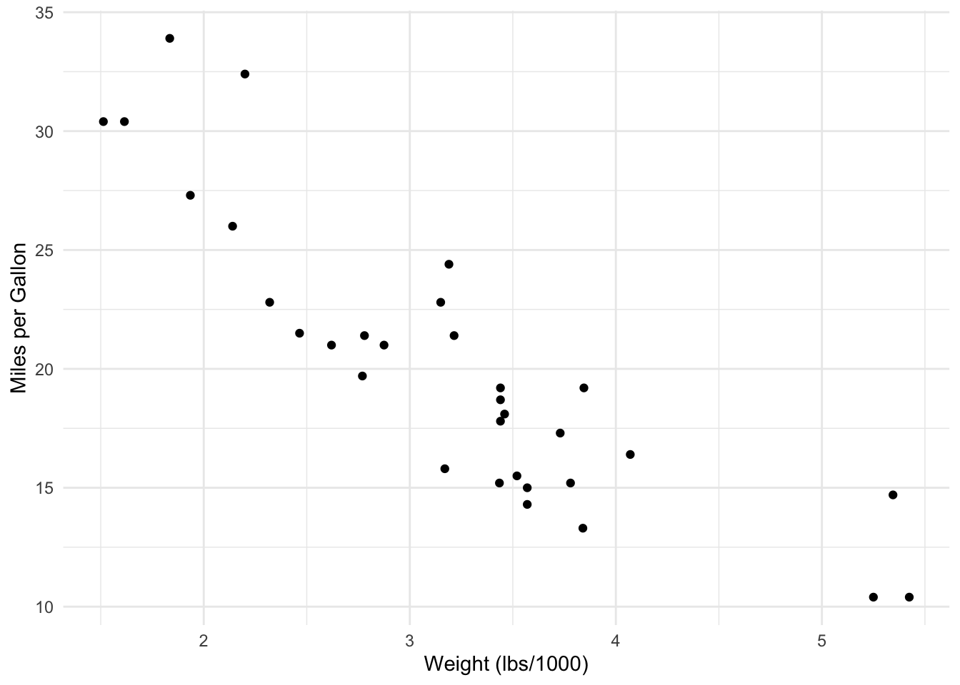
29.2.5 Step 3: Fit Models
Let us create a function so we can build multiple models. We will fit a standard linear (degree = 1) and a quadratic polynomial (degree = 2) to the mtcars dataset.
# Function to fit and evaluate polynomial regression models
fit_poly_regression <- function(degree) {
  #argument specifies the degree of the polynomial for the regression
  formula <- as.formula(paste("mpg ~ poly(wt, ", degree, ", raw = TRUE)"))
  #paste concatenates the components into a single string eg:`mpg ~ poly(wt, 2)`
  #poly returns an orthogonal polynomials as default
  #(If `raw = TRUE` calculates raw polynomial instead of orthogonal polynomial)
  #as.formula converts the constructed string into a formula object
  lm(formula, data = mtcars) #fitting the model
}

# Fit polynomial regression models with degrees 1 to 2
model_1 <- fit_poly_regression(1)
model_2 <- fit_poly_regression(2)
*Note 1: To learn more about orthogonal polynomial regression, follow: a. Orthogonal polynomial equation and explanation b. Stackoverflow - difference between raw vs orthogonal polynomial c. StackExchange - Interpreting coefficients from raw vs orthogonal polynomial
*Note 2: Using orthogonal polynomial regression would have also resulted in same plots based on which the assumptions are assessed. Moreover, it produces exact same p-value for the quadratic term but the p-value for linear term and the estimates for intercept, linear and quadratic term would be different than using raw polynomial regression.
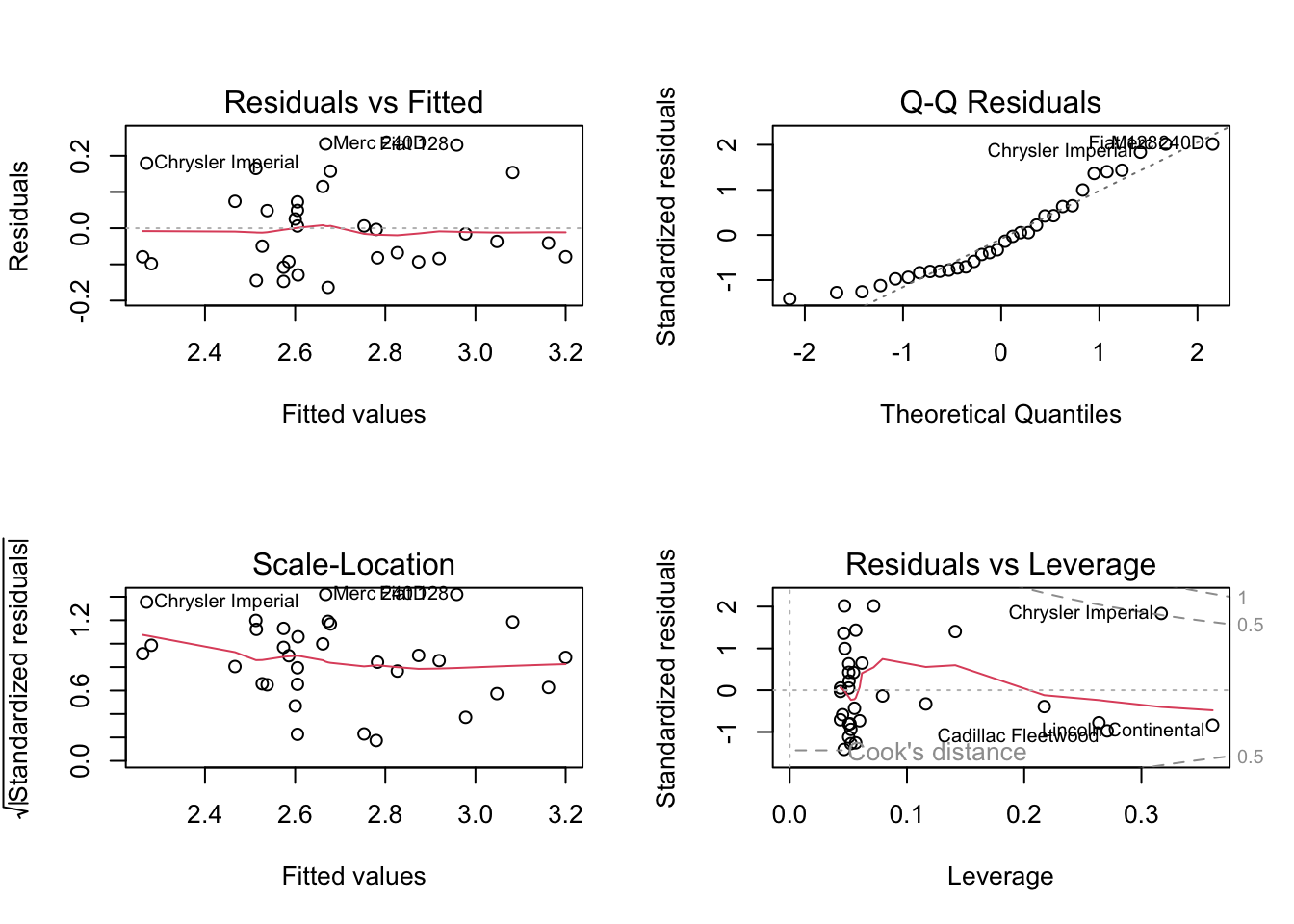
29.2.6 Step 4: Assess Assumptions
Before we can interpret the model, we have to check the assumptions. We will check these assumptions via plots:
- Residuals vs. Fitted values (used to check the linearity assumption),
- a Q-Q plot of the Residuals (used to check the normality of the residuals),
- a Scale-Location plot (used to check for heteroskedasticity), and
- Residuals vs. Leverage values (identifies overly influential values, if any exist).
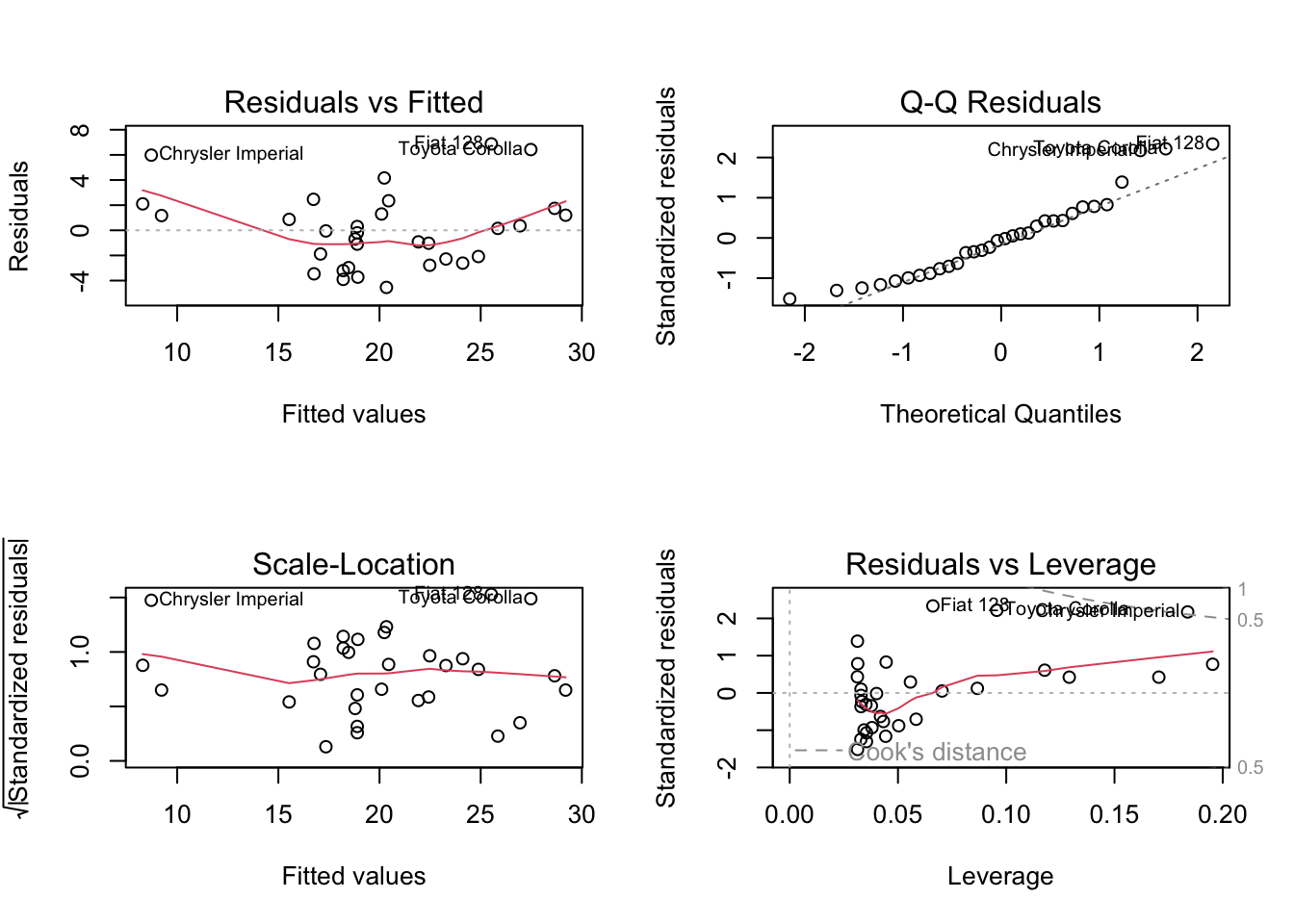
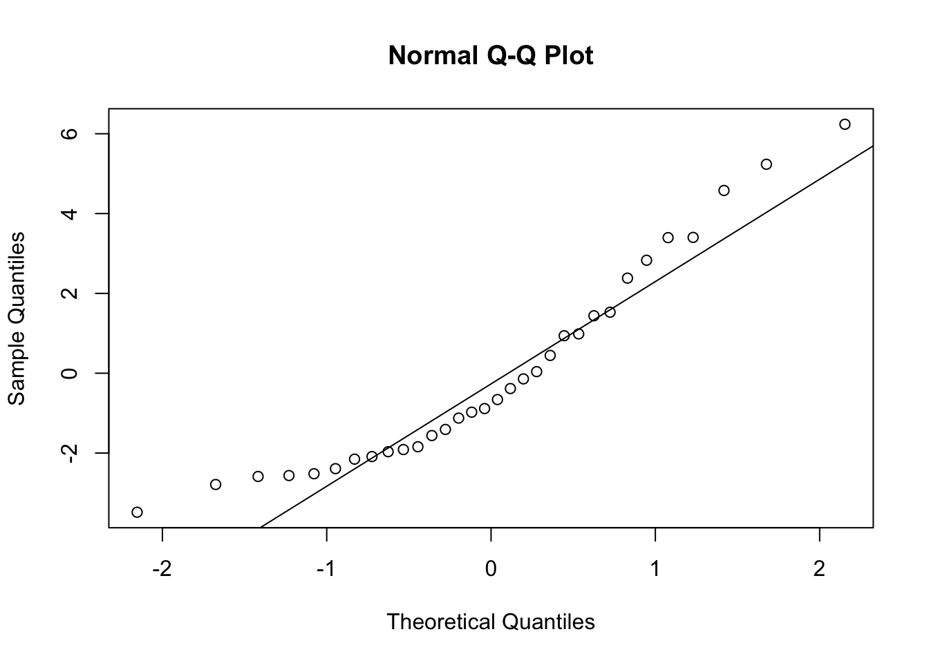
The residuals vs fitted graph in the linear model has a U-shape, which suggests that we need a quadratic polynomial component. The Q-Q plot shows that the residuals are not normally distributed, so we should take additional steps to transform the response feature (such as via a square root or log transformation, or something similar).
29.2.7 Conducting cube root transformation
We will cube root transform the response variable to build the models again.
#cube root transformation of response variable (mpg)
library(dplyr)
mtcars <- mtcars %>% mutate(mpg_cuberoot = mpg^(1/3))

#Running model after cube root transformation
fit_poly_regression_2 <- function(degree) {
  #argument specifies the degree of the polynomial for the regression
  formula_2 <- as.formula(paste("mpg_cuberoot ~ poly(wt, ", degree, ", raw = TRUE)"))
  #paste concatenates the components into a single string eg:`mpg ~ poly(wt, 2)`
  #poly returns an orthogonal polynomials as default
  #(If `raw = TRUE` calculates raw polynomial instead of orthogonal polynomial)
  #as.formula converts the constructed string into a formula object
  lm(formula_2, data = mtcars) #fitting the model
}

# Fit polynomial regression models with degrees 1 to 2
model_1_b <- fit_poly_regression_2(1)
model_2_b <- fit_poly_regression_2(2)
29.2.8 Assessing assumptions on cube root transformed data
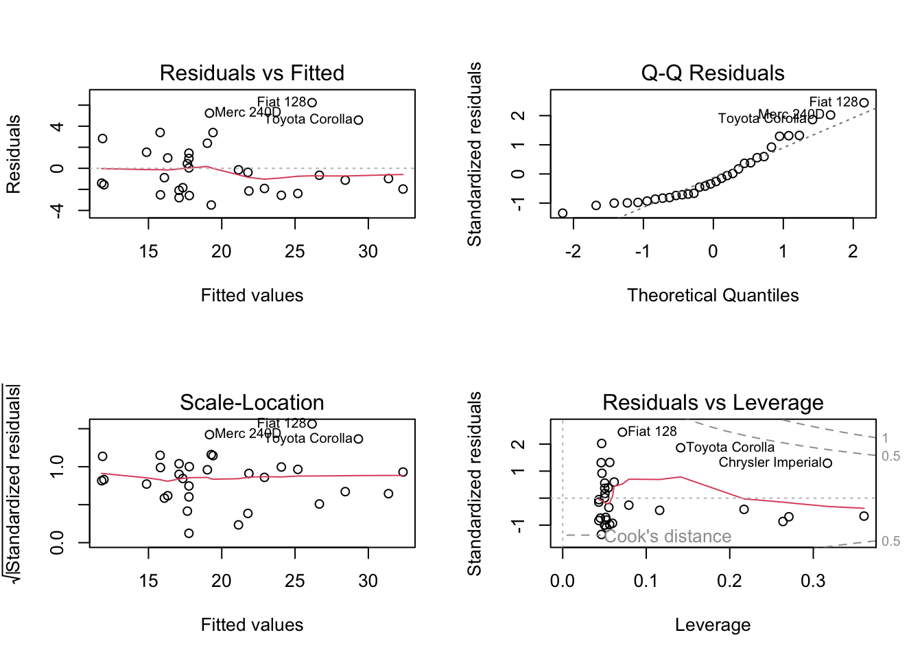
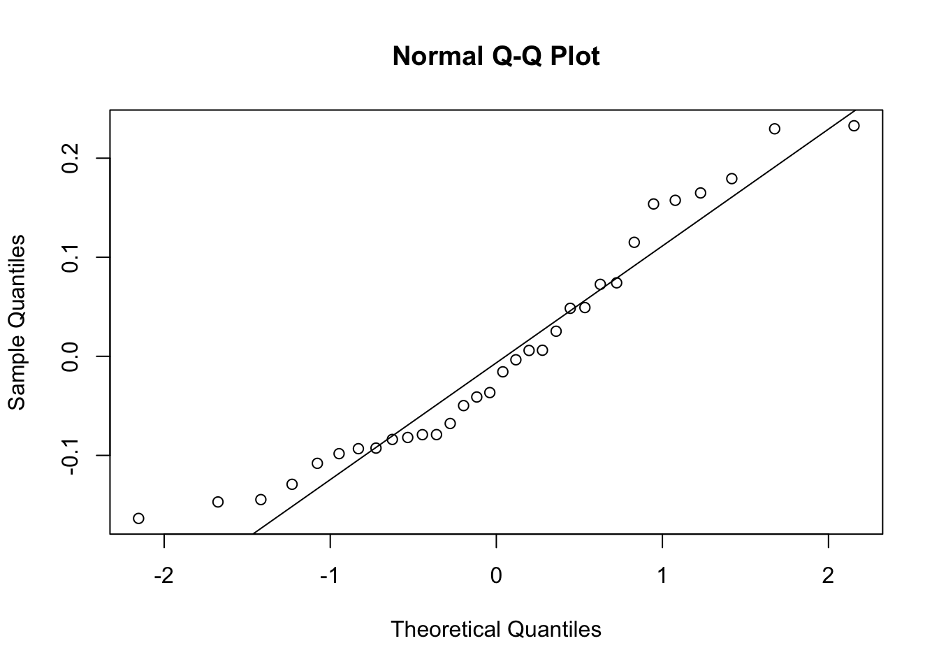
We will assess the assumption of the polynomial regression with the plots similar to non-transformed model.
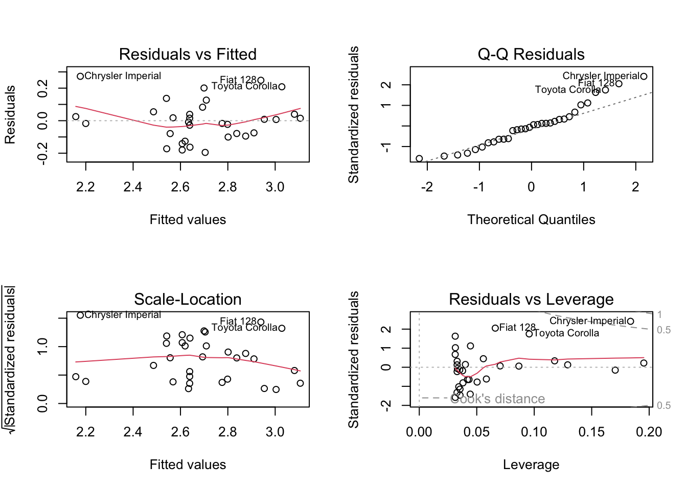
After cube root transformation of the response variable, the residuals are seem to approximately normally distributed. Zoom in to see the difference between the Q-Q plots in the first quadratic model (model_2) and cube root transformed quadratic model (model_2_b). You can also draw the Q-Q plot again to see the difference more distinctly.
29.2.9 Step 5. Describe Model Output
As the residuals of the cube root transformed model seem to be approximately normal, here is an example of how to interpret this output.
summary(model_2)
Call:
lm(formula = formula, data = mtcars)

Residuals:
   Min     1Q Median     3Q    Max
-3.483 -1.998 -0.773  1.462  6.238

Coefficients:
                         Estimate Std. Error t value Pr(>|t|)
(Intercept)               49.9308     4.2113  11.856 1.21e-12 ***
poly(wt, 2, raw = TRUE)1 -13.3803     2.5140  -5.322 1.04e-05 ***
poly(wt, 2, raw = TRUE)2   1.1711     0.3594   3.258  0.00286 **
---
Signif. codes:  0 '***' 0.001 '**' 0.01 '*' 0.05 '.' 0.1 ' ' 1

Residual standard error: 2.651 on 29 degrees of freedom
Multiple R-squared:  0.8191,    Adjusted R-squared:  0.8066
F-statistic: 65.64 on 2 and 29 DF, p-value: 1.715e-11summary(model_2_b)
Call:
lm(formula = formula_2, data = mtcars)

Residuals:
     Min       1Q   Median       3Q      Max
-0.16361 -0.08607 -0.02612  0.07303  0.23272

Coefficients:
                         Estimate Std. Error t value Pr(>|t|)
(Intercept)               3.84775    0.18784  20.484  < 2e-16 ***
poly(wt, 2, raw = TRUE)1 -0.48063    0.11214  -4.286 0.000183 ***
poly(wt, 2, raw = TRUE)2  0.03471    0.01603   2.165 0.038777 *
---
Signif. codes:  0 '***' 0.001 '**' 0.01 '*' 0.05 '.' 0.1 ' ' 1

Residual standard error: 0.1182 on 29 degrees of freedom
Multiple R-squared:  0.8171,    Adjusted R-squared:  0.8044
F-statistic: 64.76 on 2 and 29 DF,  p-value: 2.012e-11
The model could be said as being highly significant as indicated by the p-value. The significant negative linear term and significant positive quadratic term imply that mpg decreases with weight initially, but the rate of decrease slows as weight increases.
The purpose of checking the transformed response is to confirm that the confidence intervals are valid and the signs of the regression coefficients are going are correct (i.e. in the same direction) as the original model (non-transformed quadratic model).
29.2.10 Bonus Step: Visualize the Final Model
Finally, we will build the scatter plot with the polynomial regression line to visualize the fit:
# Create a data frame with data points and predictions
plot_data <- data.frame(
  wt = mtcars$wt,
  mpg = mtcars$mpg,
  mpg_predicted = predict(model_2, newdata = mtcars)
)

# Scatter plot with the polynomial regression line
ggplot(plot_data) +
  theme_minimal() +
  aes(x = wt, y = mpg) +
  labs(
    title = "Scatter Plot with Polynomial Regression Line",
    x = "Weight (wt)",
    y = "Miles per Gallon (mpg)"
  ) +
  geom_point() +
  geom_line(aes(y = mpg_predicted), color = "red", size = 1)
Warning: Using `size` aesthetic for lines was deprecated in ggplot2 3.4.0.
ℹ Please use `linewidth` instead.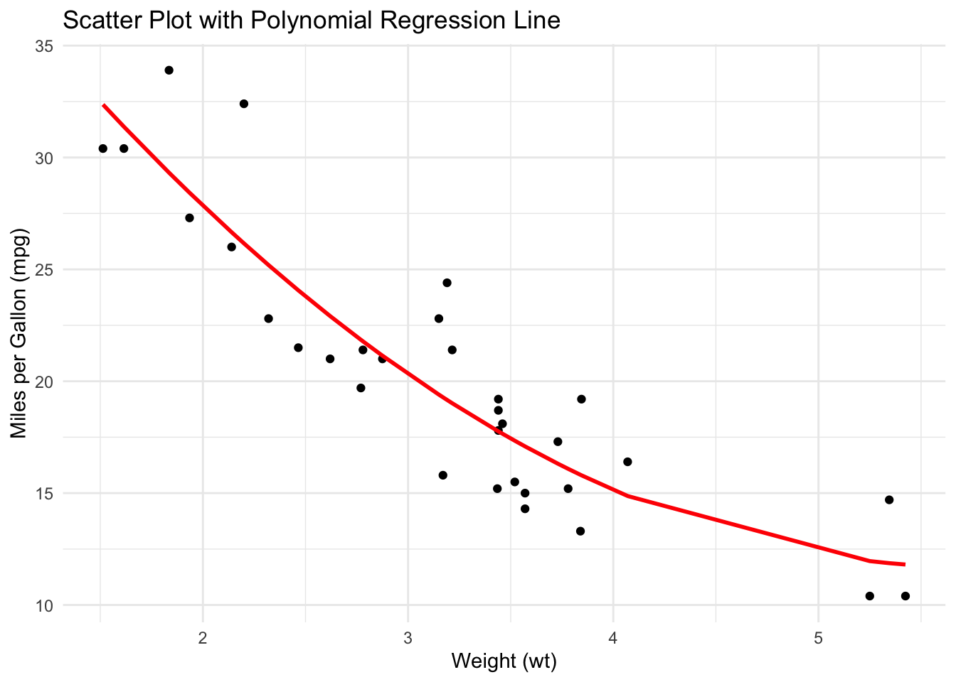
plot_data_b <- data.frame(
  wt = mtcars$wt,
  mpg_cuberoot = mtcars$mpg_cuberoot,
  mpg_predicted = predict(model_2_b, newdata = mtcars)
)

# Scatter plot with the polynomial regression line
ggplot(plot_data_b) +
  theme_minimal() +
  aes(x = wt, y = mpg_cuberoot) +
  labs(
    title = "Scatter Plot with Polynomial Regression Line (Cube transformed)",
    x = "Weight (wt)",
    y = "Cube transfomred Miles per Gallon (mpg)"
  ) +
  geom_point() +
  geom_line(aes(y = mpg_predicted), color = "red", size = 1)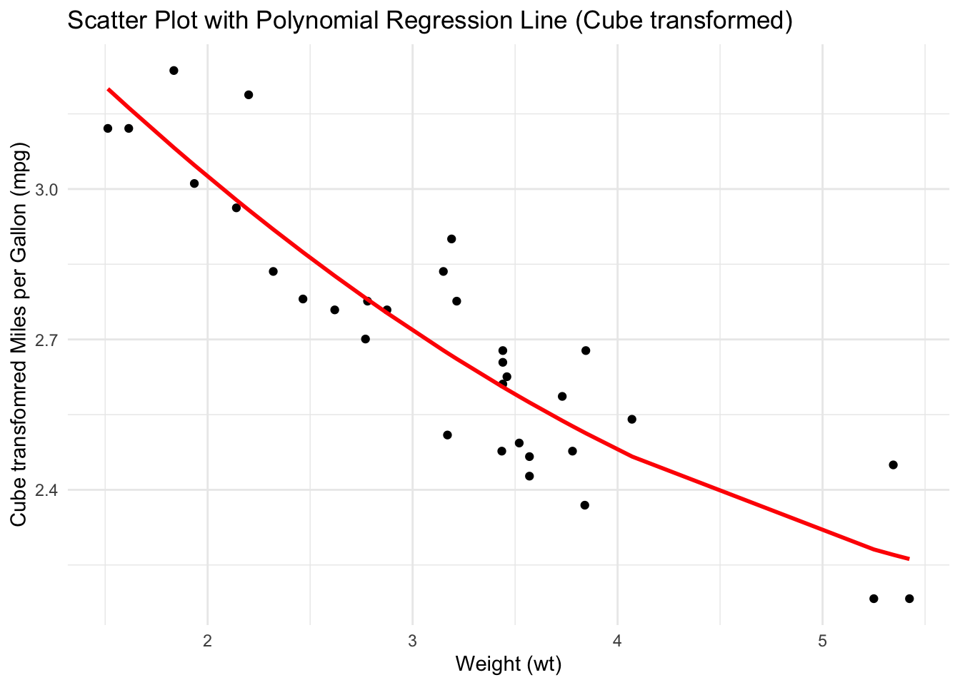
29.3 References
Field, A. (2013). Discovering Statistics Using IBM SPSS Statistics. (4th ed.). Sage Publications.
https://bookdown.org/ssjackson300/Machine-Learning-Lecture-Notes/#welcome
https://stats.libretexts.org/Bookshelves/Advanced_Statistics/Analysis_of_Variance_and_Design_of_Experiments/10%3A_ANCOVA_Part_II/10.02%3A_Quantitative_Predictors_-_Orthogonal_Polynomials#